How Good is That Random Number Generator?

Recently, I saw a reference to an interesting piece from 2013 by Peter Grogono, a computer scientist now retired from Concordia University. It's to do with checking the "quality" of a (pseudo-) random number generator.

Specifically, Peter discusses what he calls "The Pickover Test". This refers to the following suggestion that he attributes to Clifford Pickover (1995, Chap. 31):

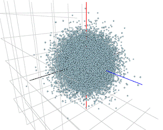
"Pickover describes a simple but quite effective technique for testing RNGs visually. The idea is to generate random numbers in groups of three, and to use each group to plot a point in spherical coordinates. If the RNG is good, the points will form a solid sphere. If not, patterns will appear. 

When it is used with good RNGs, the results of the Pickover Test are rather boring: it just draws spheres. The test is much more effective when it is used with a bad RNG, because it produces pretty pictures." 

Peter provides some nice examples of such pretty pictures!

I thought that it would be interesting to apply the Pickover Test to random numbers produced by the (default) RNG's for various distributions in R.

Before looking at the results, note that is the support of the distribution in question is finite (e.g., the Beta distribution), then the "solid sphere" that is referred to in the Pickover Test will become a "solid box". Similarly, if the support of the distribution is the real half-line (e.g., the Chi-Square distribution), the "solid sphere" will become a "solid quarter-sphere".

You can find the R code that I used on the code page that goes with this blog. Specifically, I used the "rgl" package for the 3-D plots.

Here are some of my results, in each based on a sequence of 33,000 "triplets" of random numbers:

(i) Standard Normal (using "rnorm")

(ii) Uniform on [0 , 1] (using "runif")

(iii) Binomial [n = 100, p = 0.5] (using "rbinom")

(iv) Poisson [mean = 10] (using "rpois")

(v) Standard Logistic (using "rlogis")

(vi) Beta [1 , 2] (using "rbeta")

(vii) Chi-Square [df = 5] (using "rchisq")

(vii) Student-t [df = 3] (using "rt")

(viii) Student-t [df = 7] (using "rt")

(Note that if you run my R code you can rotate the resulting 3-D plots to change the viewing aspect by holding the left mouse key and moving the mouse. You can zoom in and out by "scrolling".)

On the whole, the results look pretty encouraging, as you'd hope! One possible exception is the case of the Student-t distribution with relatively small degrees of freedom.

Of course, the Pickover "Test" is nothing more than a quick visual aid that can alert you to possible problems with your RNG. It's not intended to be a substitute for more formal, and more specific, hypothesis tests for the distribution membership, independence, etc., of your random numbers..

References

Adler, D., D. Murdoch, et al., 2017' 'rgl' package, version 0-98.1.

Pickover, C., 1995. Keys to Infinity. Wiley, New York.


© 2017, David E. Giles

Misclassification in Binary Choice Models

Several years ago I wrote a number of posts about Logit and Probit models, and the Linear Probability Model LPM). One of those posts (also, see here) dealt with the problems that arise if you mis-classify the dependent variable in such models.  That is, in the binary case, if some of your "zeroes" should be "ones", and/or vice versa.

In a conventional linear regression model, measurement errors in the dependent variable are not a biog deal. However, the situation is quite different with Logit, Probit, and the LPM.

This issue is taken up in detail in an excellent, recent, paper by Meyer and Mittag (2017), and I commend their paper to you.

To give you an indication of what those authors have to say, this is from their Introduction:

".....the literature has established that misclassification is pervasive and affects estimates, but not how it affects them or what can still be done with contaminated data. This paper characterizes the consequences of misclassification of the dependent variable in binary choice models and assesses whether substantive conclusions can still be drawn from the observed data and if so, which methods to do so work well. We first present a closed form solution for the bias in the linear probability model that allows for simple corrections. For non-linear binary choice models such as the Probit model, we decompose the asymptotic bias into four components. We derive closed form expressions for three bias components and an equation that determines the fourth component. The formulas imply that if misclassification is conditionally random, only the probabilities of misclassification are required to obtain the exact bias in the linear probability model and an approximation in the Probit model. If misclassification is related to the covariates, additional information on this relation is required to assess the (asymptotic) bias, but the results still imply a tendency for the bias to be in the opposite direction of the sign of the coefficient."

This paper includes a wealth of information, including some practical guidelines for practitioners.

Reference

Meyer, B. D. and N. Mittag, 2017. Misclassification in binary choice models. Journal of Econometrics, 200, 295-311.

© 2017, David E. Giles

Monte Carlo Simulations & the "SimDesign" Package in R

Past posts on this blog have included several relating to Monte Carlo simulation - e.g., see here, here, and here.

Recently I came across a great article by Matthew Sigal and Philip Chalmers in the Journal of Statistics Education. It's titled, "Play it Again: Teaching Statistics With Monte Carlo Simulation", and the full reference appears below.

The authors provide a really nice introduction to basic Monte Carlo simulation, using R. In particular, they contrast using a "for loop" approach, with using the "SimDesign" R package (Chalmers, 2017). 

Here's the abstract of their paper:

"Monte Carlo simulations (MCSs) provide important information about statistical phenomena that would be impossible to assess otherwise. This article introduces MCS methods and their applications to research and statistical pedagogy using a novel software package for the R Project for Statistical Computing constructed to lessen the often steep learning curve when organizing simulation code. A primary goal of this article is to demonstrate how well-suited MCS designs are to classroom demonstrations, and how they provide a hands-on method for students to become acquainted with complex statistical concepts. In this article, essential programming aspects for writing MCS code in R are overviewed, multiple applied examples with relevant code are provided, and the benefits of using a generate–analyze–summarize coding structure over the typical “for-loop” strategy are discussed."

The SimDesign package provides an efficient, and safe template for setting pretty much any Monte Carlo experiment that you're likely to want to conduct. It's really impressive, and I'm looking forward to experimenting with it.

The Sigal-Chalmers paper includes helpful examples, with the associated R code and output. It would be superfluous for me to add that here.

Needless to say, the SimDesign package is just as useful for simulations in econometrics as it is for those dealing with straight statistics problems. Try it out for yourself!

References

Chalmers, R. P., 2017. SimDesign: Structure for Organizing Monte Carlo Simulation Designs, R package version 1.7.

M. J. Sigal and R. P. Chalmers, 2016. Play it again: Teaching statistics with Monte Carlo simulation. Journal of Statistics Education, 24, 136-156.

© 2017, David E. Giles

Econometrics Reading List for September

A little belatedly, here is my September reading list:

• Benjamin, D. J. et al., 2017. Redefine statistical significance. Pre-print.
• Jiang, B., G. Athanasopoulos, R. J. Hyndman, A. Panagiotelis, and F. Vahid, 2017. Macroeconomic forecasting for Australia using a large number of predictors. Working Paper 2/17, Department of Econometrics and Business Statistics, Monash University.
• Knaeble, D. and S. Dutter, 2017. Reversals of least-square estimates and model-invariant estimations for directions of unique effects. The American Statistician, 71, 97-105.
• Moiseev, N. A., 2017. Forecasting time series of economic processes by model averaging across data frames of various lengths. Journal of Statistical Computation and Simulation, 87, 3111-3131.
• Stewart, K. G., 2017. Normalized CES supply systems: Replication of Klump, McAdam and Willman (2007). Journal of Applied Econometrics, in press.
• Tsai, A. C., M. Liou, M. Simak, and P. E. Cheng, 2017. On hyperbolic transformations to normality. Computational Statistics and Data Analysis, 115, 250-266,

© 2017, David E. Giles