My post yesterday, on Allocation Models, drew a comment to the effect that in such models the dependent variables take values that must to be non-negative fractions. Well, as I responded, that's true sometimes (e.g., in the case of market shares); but not in other cases- such as the Engel curve example that I mentioned in the post.
The anonymous comment was rather terse, but I'm presuming that the point that was intended is that if the y variables have to be positive fractions, we wouldn't want to use OLS. Ideally, that's so. Of course, we could use OLS and then check that all of the within-sample predicted values are between zero and one. Better still, we could use a more suitable estimator - one that takes the restriction on the data values into account.
The obvious solution is to assume that the errors, and hence the y values, follow a Beta distribution, and then estimate the equations by MLE. As I noted in my response to the comment, the "adding up" restictions that are needed on the parameters will be satisfied automatically, just as they are under OLS estimation.
Here's a demonstration of this.
First, consider a random variable, Y, which follows a Beta distribution, with shape parameters p and q, so that its density is:
f(y | p , q) = Γ(p + q) / [Γ(p) Γ(q)] yp - 1 (1 - y)q - 1 ; p, q > 0 ; 0 < y < 1
Now re-parameterize the distribution, using
μ = p / (p + q) ; where 0 < mu < 1
φ = (p + q) ; where phi > 0 .
The density of Y is now:
f(y | μ, φ) = Γ(φ) / [Γ(μφ) Γ(φ(1 - μ))] yμφ - 1 (1 - y)(1 - μ)φ - 1 ,
and E[Y] = μ ; var.[Y] = μ(1 - μ) / φ.
Then, following Ferrari and Cribari-Neto (2004), we can introduce regressors to explain the mean of Y. After all, this is what happens in a linear regression model, and it's also what we do in, say, a Poisson regression model. The mean will then vary from observation to observation.
Specifically, let g(μi) = xi'β , where β is a (k x 1) vector of parameters, and xi' is a row vector giving the ith. observation on each of the regressors. Various link-functions, g( . ), can be used. A particularly convenient one is the logit link:
μi = exp(xi'β) / [1 + exp(xi'β)] ; i = 1, 2, ... , n.
The ith. value for the log-likelihood function can be shown to be:
li(μi , φ) = logΓ(φ) - logΓ(μiφ) - logΓ[(1 - μi)φ] + (μiφ - 1) log(yi) + [(1 - μi)φ - 1)] log(1 - yi) .
It's then straightforward to obtain the MLEs of φ and the β elements) by numerical methods.
Let's start off where we did in the previous post, with a simple example involving a 2-equation allocation model. The regressors will just be an intercept and a single variable, x, but this simplification doesn't affect anything.
I'll assume that y1 and y2 are "share" variables, so 0 ≤ yji ≤ 1 ; for j = 1, 2 ; and i = 1, 2, ..., n. (We could change the weak inequalities to strong inequalities without affecting anything, because the y's are going to be continuous random variables.)
Also, (y1i + y2i) = 1 ; for all i. Notice that as we have an intercept in each equation, at each point in the sample, the two dependent variables sum to one of the regressors. Now, let's see what happens when we apply Beta regression to this simple allocation model.
Without going through the theory, let's consider an empirical application of MLE in the context that we're considering here. The EViews workfile and the R code that I've used are both on the code page for this blog, and the (artificial) data are available on the data page.
First, using EViews......................
I've called the intercept coefficients α1 and α2 for the two equations; and I've called the coefficients of the x regressor β1 and β2 in the two equations. φ1 and φ2 are the scale parameters.
I've created LOGL objects for each equation. The first one looks like this:
The second one has exactly the same style.
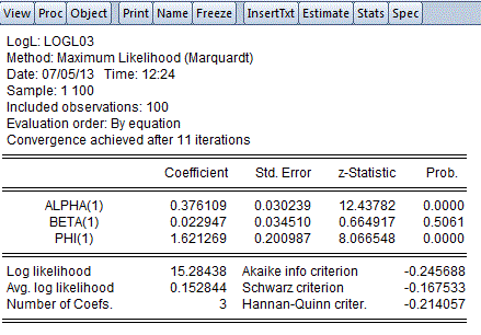
Here are MLE results for the first equation:
and
So, there we have it! You don't have to use OLS to get the "adding up" results mentioned in the previous post. You can use Beta regression and MLE to allow for the fact that the dependent variables may be "shares", and the results still hold.
I've created LOGL objects for each equation. The first one looks like this:
The second one has exactly the same style.
Here are MLE results for the first equation:
and the second equation:
Notice that the estimates of the two intercept coefficients sum to zero, and so do the estimates of the two slope coefficients. This is correct. Remember that we used the logit link function, and exp(0) = 1.
Also, notice that the estimates of the two scale parameters are the same in each equation. This corresponds to the singular covariance matrix that we saw in the earlier post. There are two equations, but only one scale parameter can be estimated freely.
What if we didn't use the logit link function, but simply specified the means as μ1i = α1 + β1xi, and μ2i = α2 + β2xi? In this case, the results we get are:
and
In this case, the intercept coefficients sum to one, the slopes sum to zero, and once again the scale parameter estimates are identical across the equations.
The predicted mean functions sum to one across the two equations, regardless of the link function we use:
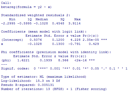
Now, let's repeat the exercise using R. Specifically we're going to use the betareg package (Cribari-Neto and Zeileis, 2010). The R code is here. Here are the results, using the logit link function:
So, there we have it! You don't have to use OLS to get the "adding up" results mentioned in the previous post. You can use Beta regression and MLE to allow for the fact that the dependent variables may be "shares", and the results still hold.
References
Ferrari, S. L. P. and F. Cribari-Neto, 2004. Beta regression for modelling rates and proportions Journal of Applied Statistics, 31, 799-815.
Cribari-Neto, F. and A. Zeileis, 2010. Beta regression in R. Journal of Statistical Software, 34(2).
© 2013, David E. Giles


Thanks for the nice post and the publicity for our R package. Note, however, that the JSS manuscript was co-authored by Francisco and myself, not Silvia.
ReplyDeleteAchim - my apologies!! Fixed now.
DeleteDG
No worries, thanks for the quick fix!
DeleteAny advice if the ratio's are a time series? What are your thoughts on including lags of each of the components as regressors with various these link functions?
ReplyDeleteOne concern would be lack of independence. Independence is assumed in the construction of the log-likelihood function used here. However, if any dependencies were incorporated properly into the specification of the likelihood function, then no problem.
DeleteDo you know if there is a code for Beta regression for STATA? I'm using the Papke and Woolridge GLM QMLE method with a logit link function, but would like to also try the Beta regression for proportional data. Particularly since I believe the Beta regression would be more applicable to smaller samples, right?
ReplyDeleteHi - no idea, as I'm not a STATA user. It's not in EViews either, but it's trivial to code up the log-likelihood function with 3 lines of code, as in my EViews workfile:
Delete@logl ll1
mu1=exp(alpha(1)+beta(1)*x )/ (1 + exp(alpha(1)+beta(1)*x))
ll1=log(@gamma(phi(1)))-log(@gamma(phi(1)*mu1))-log(@gamma(phi(1)*(1-mu1)))+(phi(1)*mu1-1)*log(y1)+(phi(1)*(1-mu1)-1)*log(1-y1)
and I know you can do the same sort of thing easily in STATA.
DG
I see..ok, thanks, I'll give it a shot!
DeleteThere is an expository paper discussing the topic for panels. We use the approach fairly often for time series analysis of allocation data. "Cake Slicing and Revealed Government Preference" Bell Journal of Economics, 1982
ReplyDeleteThank you very much! How does the model change when we are in a panel data structure, i.e. for the same year and the same country the sum of the independent variables across the equations is 1?
ReplyDeleteDo I have to perform an OLS estimation or something else?