Visualizing Random p-Values

Here's a follow-up to yesterday's post on Wolfram's CDF file format. In an earlier post (here) I discussed the fact the p-values are random variables, with their own sampling distribution.

A great way of visualizing a number of the points that I made in that post is to use the CDF file for the Mathematica app. written by Ian McLeod (University of Western Ontario). You can run it/download it from here, using Wolfram's free CDF Player (here).

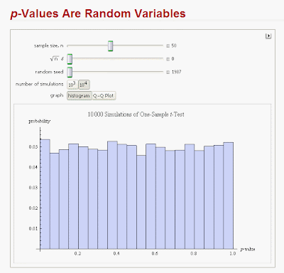
You'll recall that a p-value is uniformly distributed on [0 , 1] if the null hypothesis being tested is true. Using Ian's app., here is an example of what you see for the case where you're testing the null of a zero mean in a normal population, against a 2-sided alternative:

The null hypothesis is TRUE. The sample size is n = 50, and the simulation experiment involves 10,000 replications. You can see that the empirical distribution is approaching the Uniform true sampling distribution.

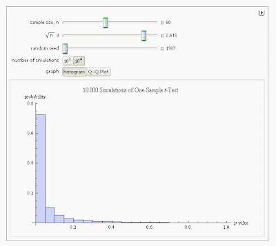
When the true mean of the distribution is 2.615 (so the null hypothesis is FALSE), the sampling distribution of the (two-sided) p-value looks like this:

If you're not sure why the pictures look like this, you might want to take a look at my earlier post, ("May I Show You My Collection of p-Values?")

© 2011, David E. Giles