Saturday, December 31, 2016

New Year's Reading

New Year's resolution - read more Econometrics!
  • Bürgi, C., 2016. What do we lose when we average expectations? RPF Working Paper No. 2016-013, Department of Economics, George Washington University.
  • Cox, D.R., 2016. Some pioneers of modern statistical theory:A personal reflection. Biometrika, 103, 747-759
  • Golden, R.M., S.S. Henley, H. White, & T.M. Kashner, 2016. Generalized information matrix tests for detecting model misspecification. Econometrics, 4, 46; doi:10.3390/econometrics4040046.
  • Phillips, G.D.A. & Y. Xu, 2016. Almost unbiased variance estimation in simultaneous equations models. Working Paper No. E2016/10, Cardiff Business School, University of Cardiff. 
  • Siliverstovs, B., 2016. Short-term forecasting with mixed-frequency data: A MIDASSO approach. Applied Economics, 49, 1326-1343.
  • Vosseler, A. & E. Weber, 2016. Bayesian analysis of periodic unit roots in the presence of a break. Applied Economics, online.
Best wishes for 2017, and thanks for supporitng this blog!

© 2016, David E. Giles

Thursday, December 29, 2016

Why Not Join The Replication Network?

I've been a member of The Replication Network (TRN) for some time now, and I commend it to you.

I received the End-of-the-Year Update for the TRN today, and I'm taking the liberty of reproducing it below in its entirety in the hope that you may consider getting involved.

Here it is:

Wednesday, December 28, 2016

More on the History of Distributed Lag Models

In a follow-up to my recent post about Irving Fisher's contribution to the development of distributed lag models,  Mike Belongia emailed me again with some very interesting material. He commented:
"While working with Peter Ireland to create a model of the business cycle based on what were mainstream ideas of the 1920s (including a monetary policy rule suggested by Holbrook Working), I ran across this note on Fisher's "short cut" method to deal with computational complexities (in his day) of non-linear relationships. 
I look forward to your follow-up post on Almon lags and hope Fisher's old, and sadly obscure, note adds some historical context to work on distributed lags."
It certainly does, Mike, and thank you very much for sharing this with us.

The note in question is titled, "Irving Fisher: Pioneer on distributed lags", and was written by J.N.M Wit (of the Netherlands central bank) in 1998. If you don't have time to read the full version, here's the abstract:
"The theory of distributed lags is that any cause produces a supposed effect only after some lag in time, and that this effect is not felt all at once, but is distributed over a number of points in time. Irving Fisher initiated this theory and provided an empirical methodology in the 1920’s. This article provides a small overview."
Incidentally, the paper co-authored with Peter Ireland that Mike is referring to it titled, "A classical view of the business cycle", and can be found here.

© 2016, David E. Giles

Tuesday, December 27, 2016

More on Orthogonal Regression

Some time ago I wrote a post about orthogonal regression. This is where we fit a regression line so that we minimize the sum of the squares of the orthogonal (rather than vertical) distances from the data points to the regression line.

Subsequently, I received the following email comment:
"Thanks for this blog post. I enjoyed reading it. I'm wondering how straightforward you think this would be to extend orthogonal regression to the case of two independent variables? Assume both independent variables are meaningfully measured in the same units."
Well, we don't have to make the latter assumption about units in order to answer this question. And we don't have to limit ourselves to just two regressors. Let's suppose that we have p of them.

In fact, I hint at the answer to the question posed above towards the end of my earlier post, when I say, "Finally, it will come as no surprise to hear that there's a close connection between orthogonal least squares and principal components analysis."

What was I referring to, exactly?

Monday, December 26, 2016

Specification Testing With Very Large Samples

I received the following email query a while back:
"It's my understanding that in the event that you have a large sample size (in my case, > 2million obs) many tests for functional form mis-specification will report statistically significant results purely on the basis that the sample size is large. In this situation, how can one reasonably test for misspecification?" 
Well, to begin with, that's absolutely correct - if the sample size is very, very large then almost any null hypothesis will be rejected (at conventional significance levels). For instance, see this earlier post of mine.

Schmueli (2012) also addresses this point from the p-value perspective.

But the question was, what can we do in this situation if we want to test for functional form mis-specification?

Schmueli offers some general suggestions that could be applied to this specific question:
  1. Present effect sizes.
  2. Report confidence intervals.
  3. Use (certain types of) charts
This is followed with an empirical example relating toauction prices for camera sales on eBay, using a sample size of n = 341,136.

To this, I'd add, consider alternative functional forms and use ex post forecast performance and cross-validation to choose a preferred functional form for your model.

You don't always have to use conventional hypothesis testing for this purpose.

Reference

Schmueli, G., 2012. Too big to fail: Large samples and the p-value problem. Mimeo., Institute of Service Science, National Tsing Hua University, Taiwan.


© 2016, David E. Giles

Irving Fisher & Distributed Lags

Some time back, Mike Belongia (U. Mississippi) emailed me as follows: 
"I enjoyed your post on Shirley Almon;  her name was very familiar to those of us of a certain age.
With regard to your planned follow-up post, I thought you might enjoy the attached piece by Irving Fisher who, in 1925, was attempting to associate variations in the price level with the volume of trade.  At the bottom of p. 183, he claims that "So far as I know this is the first attempt to distribute a statistical lag" and then goes on to explain his approach to the question.  Among other things, I'm still struck by the fact that Fisher's "computer" consisted of his intellect and a pencil and paper."
The 1925 paper by Fisher that Mike is referring to can be found here. Here are pages 183 and 184:


Thanks for sharing this interesting bit of econometrics history, Mike. And I haven't forgotten that I promised to prepare a follow-up post on the Almon estimator!

© 2016, David E. Giles

Saturday, December 24, 2016

Sunday, December 18, 2016

Not All Measures of GDP are Created Equal

A big hat-tip to one of my former grad. students, Ryan MacDonald at Statistics Canada, for bringing to my attention a really informative C.D. Howe Institute Working Paper by Philip Cross (former Chief Economic Analyst at Statistics Canada).


We all know what's meant by Gross Domestic Product (GDP), don't we? O.K., but do you know that there are lots of different ways of calculating GDP, including the six that Philip discusses in detail in his paper, namely:
  • GDP by industry
  • GDP by expenditure
  • GDP by income
  • The quantity equation
  • GDP by input/output
  • GDP by factor input
So why does this matter?

Well, for one thing - and this is one of the major themes of Philip's paper - how we view (and compute) GDP has important implications for policy-making. And, it's important to be aware that different ways of measuring GDP can result in different numbers.

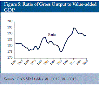
For instance, consider this chart from p.16 of the Philip's paper:


My first reaction when I saw this was "it's not flat". However, as RMM has commented below, "the line actually shows us the fluctuations of industries that are more intermediate compared with industries (or the total) that includes only final goods. Interesting and useful for business cycle analysis..."

Here's my take-away (p.18 of the paper):
"For statisticians, the different measures of GDP act as an internal check on their conceptual and empirical consistency. For economists, the different optics for viewing economic activity lead to a more profound understanding of the process of economic growth. Good analysis and policy prescription often depend on finding the right optic to understand a particular problem."
Let's all keep this in mind when we look at the "raw numbers".

© 2016, David E. Giles

Wednesday, December 14, 2016

Stephen E. Fienberg, 1942-2016

The passing of Stephen Fienberg today is another huge loss for the statistics community. Carnegie Mellon University released this obituary this morning.

Steve was born and raised in Toronto, and completed his undergraduate training in mathematics and statistics at the University of Toronto before moving to Harvard University for his Ph.D.. His contributions to statistics, and to the promotion of statistical science, were immense.

As the CMU News noted:
"His many honors include the 1982 Committee of Presidents of Statistical Society President's Award for Outstanding Statistician Under the Age of 40; the 002 ASA Samuel S. Wilks Award for his distinguished career in statistics; the first Statistical Society of Canada's Lise Manchester Award in 2008 to recognize excellence in state-of-the-art statistical work on problems of public interest; the 2015 National Institute of Statistical Sciences Jerome Sacks Award for Cross-Disciplinary Research; the 2015 R.A. Fisher Lecture Award from the Committee of Presidents of Statistical Societies and the ISBA 2016 Zellner Medal. 
Fienberg published more than 500 technical papers, brief papers, editorials and discussions.  He edited 19 books, reports and other volumes and co-authored seven books, including 1999's "Who Counts? The Politics of Census-Taking in Contemporary America," which he called "one of his proudest achievements." " 
There at least three terrific interviews with Steve that we have to remind us of the breadth of his contributions:


© 2016, David E. Giles

Monday, December 5, 2016

Monte Carlo Simulation Basics, III: Regression Model Estimators

This post is the third in a series of posts that I'm writing about Monte Carlo (MC) simulation, especially as it applies to econometrics. If you've already seen the first two posts in the series (here and here) then you'll know that my intention is to provide a very elementary introduction to this topic. There are lots of details that I've been avoiding, deliberately.

In this post we're going to pick up from where the previous post about estimator properties based on the sampling distribution left off. Specifically, I'll be applying the ideas that were introduced in that post in the context of regression analysis. We'll take a look at the properties of the Least Squares estimator in three different situations. In doing so, I'll be able to illustrate, through simulation, some "text book" results that you'll know about already.

If you haven't read the immediately preceding post in this series already, I urge you to do so before continuing. The material and terminology that follow will assume that you have.

Saturday, December 3, 2016

December Reading List

Goodness me! November went by really quickly!
 
© 2016, David E. Giles

Monday, November 28, 2016

David Hendry on "Economic Forecasting"

Today I was reading a recent discussion paper by Neil Ericcson, titled "Economic Forecasting in Theory and Practice: An Interview With David F. Hendry". The interview is to be published in the International Journal of Forecasting.

Here's the abstract:

"David Hendry has made major contributions to many areas of economic forecasting. He has developed a taxonomy of forecast errors and a theory of unpredictability that have yielded valuable insights into the nature of forecasting. He has also provided new perspectives on many existing forecast techniques, including mean square forecast errors, add factors, leading indicators, pooling of forecasts, and multi-step estimation. In addition, David has developed new forecast tools, such as forecast encompassing; and he has improved existing ones, such as nowcasting and robustification to breaks. This interview for the International Journal of Forecasting explores David Hendry’s research on forecasting."

Near the end of the wde-rangng, and thought-provoking, interview David makes the following point:
"Many top econometricians are now involved in the theory of forecasting, including Frank Diebold, Hashem Pesaran, Peter Phillips, Lucrezia Reichlin, Jim Stock, Timo Teräsvirta, KenWallis, and MarkWatson. Their technical expertise as well as their practical forecasting experience is invaluable in furthering the field. A mathematical treatment can help understand economic forecasts, as the taxonomy illustrated. Recent developments are summarized in the books by Hendry and Ericsson (2001), Clements and Hendry (2002), Elliott, Granger, and Timmermann (2006), and Clements and Hendry (2011b). Forecasting is no longer an orphan of the profession."
(My emphasis added; DG)

Neil's interview makes great reading, and I commend it to you.


© 2016, David E. Giles

Friday, November 18, 2016

The Dead Grandmother/Exam Syndrome

Anyone who's had to deal with students will be familiar with the well-known problem that biologist Mike Adams discussed in his 1999 piece, "The Dead Grandmother/Exam Syndrome", in the Annals of Improbable Research. 😊

As Mike noted,
"The basic problem can be stated very simply:
A student’s grandmother is far more likely to die suddenly just before the student takes an exam, than at any other time of year."
Based on his data, Mike observed that:
"Overall, a student who is failing a class and has a final coming up is more than 50 times more likely to lose a family member than is an A student not facing any exams. Only one conclusion can be drawn from these data. Family members literally worry themselves to death over the outcome of their relative's performance on each exam.
Naturally, the worse the student’s record is, and the more important the exam, the more the family worries; and it is the ensuing tension that presumably causes premature death."
I'll leave you to read the rest, and to find out why grandmothers are more susceptible to this problem than are grandfathers.

Enjoy Mike's research - and then make sure that you put a link to his paper on your course outlines!


© 2016, David E. Giles

Thursday, November 17, 2016

Inside Interesting Integrals

In some of my research - notably that relating to statistical distribution theory, and that in Bayesian econometrics - I spend quite a bit of time dealing with integration problems. As I noted in this recent post, integration is something that we really can't avoid in econometrics - even if it's effectively just "lurking behind the scenes", and not right in our face.

Contrary to what you might think, this can be rather interesting!

We can use software, such as Maple, or Mathematica, to help us to evaluate many complicated integrals. Of course, that wasn't always so, and in any case it's a pity to let your computer have all the fun when you could get in there and get your hands dirty with some hands-on work. Is there anything more thrilling than "cracking" a nasty looking integral?

I rely a lot on the classic book, Table of Integrals, Series and Products, by Gradshteyn Ryzhik. It provides a systematic tabulation of thousands of integrals and other functions. I know that there are zillions of books that discuss various standard methods (and non-standard tricks) to help us evaluate integrals. I'm not qualified to judge which ones are the best, but here's one that caught my attention some time back and which I've enjoyed delving into in recent months.

It's written by an electrical engineer, Paul J. Nahin, and it's called Inside Interesting Integrals.

I just love Paul's style, and I think that you will too. For instance, he describes his book in the following way -
"A Collection of Sneaky Tricks, Sly Substitutions, and Numerous Other Stupendously Clever, Awesomely Wicked, and Devilishly Seductive Maneuvers for Computing Nearly 200 Perplexing Definite Integrals From Physics, Engineering, and Mathematics. (Plus 60 Challenge Problems with Complete, Detailed Solutions.)"
Well, that certainly got my attention!

And then there's the book's "dedication":
"This book is dedicated to all who, when they read the following line from John le Carre´’s 1989 Cold War spy novel The Russia House, immediately know they have encountered a most interesting character:
'Even when he didn’t follow what he was looking at, he could relish a good page of mathematics all day long.'
as well as to all who understand how frustrating is the lament in Anthony Zee’s book Quantum Field Theory in a Nutshell:
'Ah, if we could only do the integral … . But we can’t.' "
What's not to love about that?

Take a look at Inside Interesting Integrals - it's a gem.

© 2016, David E. Giles

Saturday, November 12, 2016

Monte Carlo Simulation Basics, II: Estimator Properties

In the early part of my recent post on this series of posts about Monte Carlo (MC) simulation, I made the following comments regarding its postential usefulness in econometrics:
".....we usually avoid using estimators that are are "inconsistent". This implies that our estimators are (among other things) asymptotically unbiased. ......however, this is no guarantee that they are unbiased, or even have acceptably small bias, if we're working with a relatively small sample of data. If we want to determine the bias (or variance) of an estimator for a particular finite sample size (n), then once again we need to know about the estimator's sampling distribution. Specifically, we need to determine the mean and the variance of that sampling distribution. 
If we can't figure the details of the sampling distribution for an estimator or a test statistic by analytical means - and sometimes that can be very, very, difficult - then one way to go forward is to conduct some sort of MC simulation experiment."
Before proceeding further, let's recall just what we mean by a "sampling distribution". It's a very specific concept, and not all statisticians agree that it's even an interesting one.

Tuesday, November 8, 2016

Monte Carlo Simulation Basics, I: Historical Notes

Monte Carlo (MC) simulation provides us with a very powerful tool for solving all sorts of problems. In classical econometrics, we can use it to explore the properties of the estimators and tests that we use. More specifically, MC methods enable us to mimic (computationally) the sampling distributions of estimators and test statistics in situations that are of interest to us. In Bayesian econometrics we use this tool to actually construct the estimators themselves. I'll put the latter to one side in what follows.

Sunday, November 6, 2016

The BMST Package for Gretl

As a follow-up to this recent post, I heard again from Artur Tarassow.

You'll see from his email message below that he's extended his earlier work and has prepared a new package for Gretl called "Binary Models Specification Tests".

It's really good to see tests of this type being made available for users of different software - especially free software such as Gretl.

Artur writes:

Saturday, November 5, 2016

Snakes in a Room

Teachers frequently use analogies when explaining new concepts. In fact, most people do. A good analogy can be quite eye-opening.

The other day my wife was in the room while I was on the 'phone explaining to someone why we often like to apply BOTH the ADF test and the KPSS test when we're trying to ascertain whether a partcular time-series is stationary or non-stationary. (More specifically, whether it is I(0) or I(1).) The conversation was, not surprisingly, relatively technical in nature.

After the call was over, it occurred to me that my wife (who is an artist, and not an econometrician) might ask me what the heck all that gobbly-gook was all about. As it happened, she didn't - she had more important things on her mind, no doubt. But it forced me to think about a useful analogy that one might use in this particular instance.

I'm not suggesting that what I came up with is the best possible analogy, but for what it's worth I'll share it with you.

Friday, November 4, 2016

November Reading

You'll see that this month's reading list relates, in part, to my two recent posts about Ted Anderson and David Cox.
  • Acharya, A., M. Blackwell, & M. Sen, 2015. Explaining causal findings without bias: Detecting and assessing direct effects. RWP15-194, Harvard Kennedy School.
  • Anderson, T.W., 2005. Origins of the limited information maximum likelihood and two-stage least squares estimators. Journal of Econometrics, 127, 1-16.
  • Anderson, T.W. & H. Rubin, 1949. Estimation of the parameters of a single equation in a complete system of stochastic equations. Annals of Mathematical Statistics, 20, 46-63.
  • Cox, D.R., 1972. Regression models and life-tables (with discussion). Journal of the Royal Statistical Society B, 34, 187–220.
  • Malsiner-Walli, G. & H. Wagner, 2011. Comparing spike and slab priors for Bayesian variable selection. Austrian Journal of Statistics, 40, 241-264.
  • Psaradakis, Z. & M. Vavra, 2016. Portmanteau tests for linearity of stationary time series. Working Paper 1/2016, National Bank of Slovakia.
© 2016, David E. Giles

Thursday, November 3, 2016

T. W. Anderson: 1918-2016

Unfortunately, this post deals with the recent loss of one of the great statisticians of our time - Theodore (Ted) W. Anderson.

Ted passed away on 17 September of this year, at the age of 98.

I'm hardly qualified to discuss the numerous, path-breaking, contributions that Ted made as a statistician. You can read about those in De Groot (1986), for example.

However, it would be remiss of me not to devote some space to reminding readers of this blog about the seminal contributions that Ted Anderson made to the development of econometrics as a discipline. In one of the "ET Interviews", Peter Phillips talks with Ted about his career, his research, and his role in the history of econometrics.  I commend that interview to you for a much more complete discussion than I can provide here.

(See this post for information about other ET Interviews).

Ted's path-breaking work on the estimation of simultaneous equations models, under the auspices of the Cowles Commission, was enough in itself to put him in the Econometrics Hall of Fame. He gave us the LIML estimator, and the Anderson and Rubin (1949, 1950) papers are classics of the highest order. It's been interesting to see those authors' test for over-identification being "resurrected" recently by a new generation of econometricians. 

There are all sorts of other "snippets" that one can point to as instances where Ted Anderson left his mark on the history and development of econometrics.

For instance, have you ever wondered why we have so many different tests for serial independence of regrsssion errors? Why don't we just use the uniformly most powerful (UMP) test and be done with it? Well, the reason is that no such test (against the alternative of a first-oder autoregresive pricess) exists.

That was established by Anderson (1948), and it led directly to the efforts of Durbin and Watson to develop an "approximately UMP test" for this problem.

As another example, consider the "General-to-Specific" testing methodology that we associate with David Hendry, Grayham Mizon, and other members of the (former?) LSE school of thought in econometrics. Why should we "test down", and not "test up" when developing our models? In other words, why should we start with the most  general form of the model, and then successively test and impose restrictions on the model, rather than starting with a simple model and making it increasingly complex? The short answer is that if we take the former approach, and "nest" the successive null and alternative hypotheses in the appropriate manner, then we can appeal to a theorem of Basu to ensure that the successive test statistics are independent. In turn, this means that we can control the overall significance level for the set of tests to what we want it to be. In contrast, this isn't possible if we use a "Simple-to-General" testing strategy.

All of this spelled out in Anderson (1962) in the context of polynomial regression, and is discussed further in Ted's classic time-series book (Anderson, 1971). The LSE school referred to this in promoting the "General-to-Specific" methodology.

Ted Anderson published many path-breaking papers in statistics and econometrics and he wrote several books - arguably, the two most important are Anderson (1958, 1971). He was a towering figure in the history of econometrics, and with his passing we have lost one of our founding fathers.

References

Anderson, T.W., 1948. On the theory of testing serial correlation. Skandinavisk Aktuarietidskrift, 31, 88-116.

Anderson, T.W., 1958. An Introduction to Multivariate Statistical Analysis. WIley, New York (2nd. ed. 1984).

Anderson, T.W., 1962. The choice of the degree of a polynomial regression as a multiple decision problem. Annals of Mathematical Statistics, 33, 255-265.

Anderson, T.W., 1971. The Statistical Analysis of Time Series. Wiley, New York.

Anderson, T.W. & H. Rubin, 1949. Estimation of the parameters of a single equation in a complete system of stochastic equations. Annals of Mathematical Statistics, 20, 46-63.

Anderson, T.W. & H. Rubin, 1950. The asymptotic properties of the parameters of a single equation in a complete system of stochastic equations. Annals of Mathematical Statistics, 21,570-582.

De Groot, M.H., 1986. A Conversation with T.W. Anderson: An interview with Morris De Groot. Statistical Science, 1, 97–105.

© 2016, David E. Giles

I Was Just Kidding......!

Back in 2011 I wrote a post that I titled, "Dummies for Dummies". It began with the suggestion that I'd written a book of that name, and it included this mock-up of the "cover":


(Thanks to former grad. student, Jacob Schwartz, for helping with the pic.)

Although I did say, "O.K., I'm (uncharacteristically) exaggerating just a tad", apparently a few people took me too seriously/literally. I've had a couple of requests for the book, and even one of my colleagues asked me when it would be appearing.

Sadly, no book was ever intended - somehow, I just don't think there's the market for it!

© 2016, David E. Giles

Wednesday, November 2, 2016

Specification Tests for Logit Models Using Gretl

In various earlier posts I've commented on the need for conducting specification tests when working with Logit and Probit models. (For instance, see herehere, and here.) 

One of the seminal references on this topic is Davidson and MacKinnon (1984). On my primary website, you can find a comprehensive list of other related references, together with EViews files that will enable you to conduct various specification tests with LDV  models.

The link for that material is here.

Today I had an email from Artur Tarassow at the University of Hamburg. He wrote:
I know that you're already aware of the open-source econometric software called "Gretl". 
I would like to let you know that I updated my package "LOGIT_HETERO.gfn". This package runs both the tests of homoskedasticity and correct functional form based on your nice program "Logit_hetero.prg" written for EViews.
If you want to have a look at it, simply run:
    set echo off
    set messages off
    install LOGIT_HETERO.gfn
    include LOGIT_HETERO.gfn
    open http://web.uvic.ca/~dgiles/downloads/binary_choice/Logistic_Burr.wf1
    logit Y 0 X1 X2
    matrix M = LOGIT_HETERO(Y,$xlist,$coeff,1)
    print M
Thanks for this, Artur - I'm sure it will be very helpful to many readers of this blog.

Footnote: See Artur's comment below, and the more recent post here. In particular, note Artur's comment: As a note to your blog readers: The two Logit model related packages “logit_burr.gfn” and “LOGIT_HETERO.gfn” are not available any more, as BMST includes both of them.

Reference

Davidson, R. & J. G. MacKinnon, 1984. Convenient specification tests for logit and probit models. Journal of Econometrics, 25, 241 262.

© 2016, David E. Giles

Tuesday, November 1, 2016

International Prize in Statistics


A few days ago, the inaugural winner of the biennial International Prize in Statistics was announced.

The first recipient of the new award is Sir David Cox, whose work is, of course, well known to econometricians.

The award was made to Sir David for his "Survival Analysis Model Applied in Medicine, Science, and Engineering".

Sunday, October 2, 2016

Some Suggested Reading for October

For your enjoyment:
  • Diebold, F. X. & M. Shin, 2016. Assessing point forecast accuracy by stochastic error distance. NBER Working Paper No.2516.
  • Franses, P.H., 2016. Yet another look at MIDAS regression. Econometric Institute Report 2016-32.
  • Hillier, G. & F. Martellosio, 2016. Exact properties of the maximum likelihood estimator in spatial autoregressive models. Discussion Paper DP 07/16, Department of Economics, University of Surrey.
  • Li, L., M.J. Holmes, & B.S. Lee, 2016. The asymmetric relationship between executive earnings management and compensation: A panel threshold regression approach. Applied Economics, 48, 5525-5545. 
  • Lütkepohl, H., A. Staszewska-Bystrova, & P. Winker, 2016. Calculating joint confidence bands for impulse response functions using highest density regions. MAGKS Joint Discussion Paper 16-2016.
  • Segnon, M., R. Gupta, S. Bekiros, & M.E. Wohar, 2016. Forecasting U.S. GNP growth: The role of uncertainty. Working Paper 2016-67, Department of Economics, University of Pretoria.

© 2016, David E. Giles

Friday, September 9, 2016

Spreadsheet Errors

Five years ago I wrote a post titled, "Beware of Econometricians Bearing Spreadsheets". 

The take-away message from that post was simple: there's considerable, well-documented, evidence that spreadsheets are very, very, dangerous when it comes to statistical calculations. That is, if you care about getting the right answers!

Read that post, and the associated references, and you'll see what I mean.

(You might also ask yourself, why would I pay big bucks for commercial software that is of questionable quality when I can use high-quality statistical software such as R, for free?)

This week, a piece in The Economist looks at the shocking record of publications in genomics that fall prey to spreadsheet errors. It's a sorry tale, to be sure. I strongly recommend that you take a look.

Yes, any software can be mis-used. Anyone can make a mistake. We all know that. However, it's not a good situation when a careful and well-informed researcher ends up making blunders just because the software they trust simply isn't up to snuff!  


© 2016, David E. Giles

Friday, September 2, 2016

Dummies with Standardized Data

Recently, I received the following interesting email request:
"I would like to have your assistance regarding a few questions related to regression with standardized variables and a set of dummy variables. First of all, if the variables are standardized (xi-x_bar)/sigma, can I still run the regression with a constant? And, if my dummy variables have 4 categories, do I include all of them without the constant? Or just three and keep the constant in the regression? And, how do we interpret the coefficients of the dummy variables in such as case? I mean, idoes the conventional interpretation in a single OLS regression still apply?"

Here's my (brief) email response:
"If all of the variables (including the dependent variable) have been standardized then in general there is no need to include an intercept - in fact the OLS estimate of its coefficient will be zero (as it should be).
However, if you have (say) 4 categories in the data that you want to allow for with dummy variables, then the usual results apply:
1. You can include all 4 dummies (but no intercept). The estimated coefficients on the dummies will sum to zero with standardized data. Each separate coefficient gives you the deviation from zero for the intercept in each category.
OR (equivalently)
2. You can include an intercept and any 3 of the dummies. Again, the estimated coefficients of the dummies and the intercept will sum to zero. Suppose that you include the intercept and the dummies D2, D3, and D4. The estimated coefficient of the intercept gives you the intercept effect for category 1. The estimated coefficient for D2 gives you the deviation of the intercept for category 2, from that for category 1, etc."
You can easily verify this by fitting a few OLS regressions, and there's a lot more about regression analysis with standardized data in this earlier post of mine.


© 2016, David E. Giles

Wednesday, August 31, 2016

September Reading

Here are a few suggestions for some interesting reading this month:
© 2016, David E. Giles

Tuesday, July 26, 2016

The Forecasting Performance of Models for Cointegrated Data

Here's an interesting practical question that arises when you're considering different forms of econometric models for forecasting time-series data:
"Which type of model will perform best when the data are non-stationary, and perhaps cointegrated?"
To answer this question we have to think about the alternative models that are available to us; and we also have to decide on what we mean by 'best'. In other words, we have to agree on some sort of loss function or performance criterion for measuring forecast quality.

Notice that the question I've posed above allows for the possibility that the data that we're using are integrated, and the various series we're working with may or may not be cointegrated. This scenario covers a wide range of commonly encountered situations in econometrics.

In an earlier post I discussed some of the basic "mechanics" of forecasting from an Error Correction Model. This type of model is used in the case where our data are non-stationary and cointegrated, and we want to focus on the short-run dynamics of the relationship that we're modelling. However, in that post I deliberately didn't take up the issue of whether or not such a model will out-perform other competing models when it comes to forecasting.

Let's look at that issue here.

Tuesday, July 5, 2016

Recommended Reading for July

Now that the Canada Day and Independence Day celebrations are behind (some of) us, it's time for some serious reading at the cottage. Here are some suggestions for you:


© 2016, David E. Giles

Saturday, June 25, 2016

Choosing Between the Logit and Probit Models

I've had quite a bit say about Logit and Probit models, and the Linear Probability Model (LPM), in various posts in recent years. (For instance, see here.) I'm not going to bore you by going over old ground again.

However, an important question came up recently in the comments section of one of those posts. Essentially, the question was, "How can I choose between the Logit and Probit models in practice?"

I responded to that question by referring to a study by Chen and Tsurumi (2010), and I think it's worth elaborating on that response here, rather than leaving the answer buried in the comments of an old post.

So, let's take a look.

Tuesday, June 7, 2016

The ANU Tapes of the British (Econometrics) Invasion

As far as I know, the Beatles never performed at the Australian National University (the ANU). But the "fab. three" certainly did, and we're incredibly lucky to have the visual recordings to prove it!

Stan Hurn (Chair of the Board of the National Centre for Econometric Research, based in the Business School at the Queensland University of Technology) contacted me recently about a fantastic archive that has been made available.

The Historical Archive at the NCER now includes the digitized versions of the movies that were made in the 1970's and 1980's when various econometricians from the London School of Economics visited and lectured at the ANU. Specifically, eight lectures by Grayham Mizon, five by Ken Wallis, and a further eight lectures by Denis Sargan can be viewed here.

I was on faculty at Monash University at the time of these visits (and that of David Hendry - so I guess the fab. four of of the LSE did actually make it). I recall them well because the visitors also gave seminars in our department while they were in Australia. 

Before you view the lectures - and I really urge you to do so - it's essential that you read the background piece, "The ANU Tapes: A Slice of History", written by Chris Skeels. (Be sure to follow the "Read more" link, and read the whole piece.) As it happens, Chris was a grad. student in our group at Monash back in the day, and his backgrounder outlines a remarkable story of how the tapes were saved.

Kudos to Stan and his colleagues for putting this archive together. And double kudos to Chris Skeels for having the foresight, energy, and determination to ensure that we're all able to share these remarkable lectures.

Thank you both!

© 2016, David E. Giles

Thursday, June 2, 2016

Econometrics Reading List for June

Here's some suggested reading for the coming month:


© 2016, David E. Giles

Saturday, May 28, 2016

Forecasting From an Error Correction Model

Recently, a reader asked about generating forecasts from an estimated Error Correction Model (ECM). Really, the issues that arise are no different from those associated with any dynamic regression model. I talked about the latter in a previous post in 2013.

Anyway, let's take a look at the specifics.........

Sunday, May 22, 2016

A Quick Illustration of Pre-Testing Bias

The statistical and econometric literature on the properties of "preliminary-test" (or "pre-test") estimation strategies is large and well established. These strategies arise when we proceed in a sequential manner when drawing inferences about parameters. 

A simple example would be where we fit a regression model; test if a regressor is significant or not; and then either retain the model, or else remove the (insignificant) regressor and re-estimate the (simplified) model.

The theoretical literature associated with pre-testing is pretty complex. However, some of the basic messages arising from that literature can be illustrated quite simply. Let's look at the effect of "pre-testing" on the bias of the OLS regression estimator.

Monday, May 16, 2016

Graduate Econometrics Exam

Occasionally readers ask about the exams that I set in my graduate econometrics courses.

The elective graduate econometrics course that I taught this past semester was one titled "Themes in Econometrics". The topics that are covered vary from year to year. However, as the title suggests, the course focuses on broad themes that arise in econometrics. Examples might include maximum likelihood estimation and the associated testing strategies;instrumental variables/GMM estimation; simulation methods; nonparametric inference; and Bayesian inference.

This year most of the course was devoted to maximum likelihood, and Bayesian methods in econometrics.

The mid-term test covered the first of these two thematic topics, while the final exam was devoted largely to Bayesian inference.

You can find the mid-term test here. The final exam question paper is here; and the associated R code is here.


© 2016, David E. Giles

Sunday, May 8, 2016

Econometric Computing in the Good Ol' Days

I received an email from Michael Belongia, who said:

"I wrote earlier in response to your post about Almon lags but forgot to include an anecdote that may be of interest to your follow-up.
In the late 1960s, the "St. Louis Equation"  became a standard framework for evaluating the relative effects of monetary and fiscal policy. The equation was estimated by the use of Almon lags (see, e.g., footnotes 12 and 18 in the article).  To estimate the equation, however, the St. Louis Fed had to use the computing power of nearby McDonnell-Douglas!!!  As Keith Carlson, who was in the Bank's Research Dept at the time, confirmed for me:   
'We did send our stuff out to McDonnell-Douglas.  Gave the instructions to the page who took it to the Cotton Belt building at 4th and Pine and the output would be picked up a couple days later. We did this until about 67 or 68 when we shifted to in-house.  In fact we hired the programmer from M-D.'
Difficulties like this certainly made economists of the era think more carefully about their models before taking them to the data."
I concur wholeheartedly with Michael's last comment. My own computing experience began in the late 1960's - I've posted about this in the past in The Monkey Run.

And I haven't forgotten the follow-up post on Almon distributed lag models that I promised!

© 2016, David E. Giles

Friday, May 6, 2016

May Reading List

Here's my reading list for May:
  • Hayakawa, K., 2016. Unit root tests for short panels with serially correlated errors. Communications in Statistics - Theory and Methods, in press.
  • Hendry, D. F. and G. E. Mizon, 2016. Improving the teaching of econometrics. Discussion Paper 785, Department of Economics, University of Oxford.
  • Hoeting, J. A., D. Madigan, A. E. Raftery, and C. T. Volinsky, 1999. Bayesian model averaging: A tutorial (with comments and rejoinder). Statistical Science, 14, 382-417. 
  • Liu, J., D. J. Nordman, and W. Q. Meeker, 2016. The number of MCMC draws needed to compute Bayeian credible bounds. American Statistician, in press.
  • Lu, X., L. Su, and H. White, 2016. Granger causality and structural causality in cross-section and panel data. Working Paper No, 04-2016, School of Economics, Singapore Management University.
  • Nguimkeu, P., 2016.  An improved selection test between autoregressive and moving average disturbances in regression models. Journal of Time Series Econometrics, 8, 41-54.

© 2016, David E. Giles

Wednesday, May 4, 2016

My Latest Paper About Dummy Variables

Over the years I've posted a number of times about various aspects of using dummy variables in regression models. You can use the "Search" window in the right sidebar of this page if want to take a look at those posts.

One of my earlier working papers on this topic has now been accepted for publication.

The paper is titled, "On the Inconsistency of Instrumental Variables Estimators for the Coefficients of Certain Dummy Variables". Here's the abstract:
"In this paper we consider the asymptotic properties of the Instrumental Variables (IV) estimator of the parameters in a linear regression model with some random regressors, and other regressors that are dummy variables. The latter have the special property that the number of non-zero values is fixed, and does not increase with the sample size. We prove that the IV estimator of the coefficient vector for the dummy variables is inconsistent, while that for the other regressors is weakly consistent under standard assumptions. However, the usual estimator for the asymptotic covariance matrix of the I.V. estimator for all of the coefficients retains its usual consistency. The t-test statistics for the dummy variable coefficients are still asymptotically standard normal, despite the inconsistency of the associated IV coefficient estimator. These results extend the earlier results of Hendry and Santos (2005), which relate to a fixed-regressor model, in which the dummy variables are non-zero for just a single observation, and OLS estimation is used".
You can download the final working paper version of the paper from here.

The paper will be appearing in an upcoming issue of Journal of Quantitative Economics.


© 2016, David E. Giles

Monday, April 11, 2016

Improved Analytic Bias Correction for MLE's

Ryan Godwin and I have a new paper - "Improved Analytic Bias Correction for Maximum Likelihood Estimators". You can download it from here. (This is a revised version, 19 July 2017.)

This paper proposes a modification of the Cox-Snell/Cordeiro-Klein bias correction technique that we've used in our earlier research (including work with Helen Feng and Jacob Schwartz). For some more information about that work, see this earlier post.

© 2016, David E. Giles

Friday, April 8, 2016

The Econometric Game Winners

The results of the 2016 edition of The Econometric Game are now out:

1st. Place: Harvard University
2nd. Place: Warsaw School of Economics
3rd. Place: Erasmus University

Congratulations to all of the competitors, and to the organisers of this important event!

© 2016, David E. Giles

The Econometric Game Finalists

The Econometric Game is drawing to a close for 2016. With just hours to go the teams that are completing the final round of the competition are:

Lund University
Warsaw School of Economics
McGill University     (go Canada!)
University of Copenhagen
ENSAE
Aarhus University
Erasmus Universiteit Rotterdam
Harvard University
University of Rome Tor Vergata
University of Antwerp

The case for this year's event is discussed here.

© 2016, David E. Giles

Wednesday, April 6, 2016

The Econometric Game - Update

From the website of The Econometric Game

Revealing of the Econometric Game Case.
Today at the grand opening of the Econometric Game:
The case makers have revealed this year's theme: Socioeconomic inequity in health care use among elderly Europeans.
The case makers Pilar García-Gómez and Teresa Bago d'Uva have worked very hard on designing the case and are looking forward to the results of the participating students. Tomorrow evening the finalist will be announced.

© 2016, David E. Giles

Monday, April 4, 2016

The Econometric Game, 2016

Last December I posted about the upcoming 2016 round of The Econometric Game.

You'll find links in that post to other posts in previous years.

Well, the Game is almost up on us. If you're not familiar with it, here's the overview from  the EG website:
"Every year, the University of Amsterdam is hosting the Econometric Game, one of the most prestigious projects organized by the study association for Actuarial Science, Econometrics & Operational Research (VSAE) of the University of Amsterdam. The participating universities are expected to send delegations of four students majoring in econometrics or relevant studies with a maximum of two PhD students. The teams will be given a case study, which they will have to resolve in two days. After these two days the ten teams with the best solutions will continue to day three. On the third day the finalists have to solve a second case while the other teams can go sightseeing in Amsterdam. After the teams have explored the city, the Econometric Game Congress takes place. There are different interesting lecturers, who will speech about the case and the econometric methods necessary for solving the case. The solutions will be reviewed by a jury of qualified and independent professors and they will announce the winner of the Game. 
The Econometric Game 2016 will take place on the 6th, 7th and 8th of April 2016 in Amsterdam."

I'll comment on the results in due course.

© 2016, David E. Giles

Friday, April 1, 2016

My new Paper

I'm really pleased with the way that my recent paper (with co-author Al Gol) turned out. It's titled "HotGimmer: Random Information", and you can download it here.

Comments are welcomed, of course..........

© 2016, David E. Giles

Saturday, March 26, 2016

Who was Shirley Almon?

How often have you said to yourself, "I wonder what happened to Jane X"? (Substitute any person's name you wish.)

Personally, I've noticed a positive correlation between my age and the frequency of occurrence of this event, but we all know that correlation doesn't imply causality.

Every now and then, over the years, I've wondered what happened to Shirley Almon, of the "Almon Distributed Lag Model" fame. Of course I should have gone to the internet for assistance, but somehow, I never did this - until the other day.......

Friday, March 25, 2016

MIDAS Regression is Now in EViews

The acronym, "MIDAS", stands for several things. In the econometrics literature it refers to "Mixed-Data Sampling" regression analysis. The term was coined by Eric Ghysels a few years ago in relation to some of the novel work that he, his students, and colleagues have undertaken. See Ghysels et al. (2004).

Briefly, a MIDAS regression model allows us to "explain" a (time-series) variable that's measured at some frequency, as a function of current and lagged values of a variable that's measured at a higher frequency. So, for instance, we can have a dependent variable that's quarterly, and a regressor that's measured at a monthly, or daily, frequency.

There can be more than one high-frequency regressor. Of course, we can also include other regressors that are measured at the low (say, quarterly) frequency, as well as lagged values of the dependent variable itself. So, a MIDAS regression model is a very general type of autoregressive-distributed lag model, in which high-frequency data are used to help in the prediction of a low-frequency variable.

There's also another nice twist.......

Tuesday, March 1, 2016

March Reading List

Now is a good time to catch up on some Econometrics reading. Here are my suggestions for this month:

  • Carrasco, M. and R. Kotchoni, 2016. Efficient estimation using the characteristic function. Econometric Theory, in press.
  • Chambers, M. J., 2016. The estimation of continuous time models with mixed frequency data. Discussion Paper No. 777, Department of Economics, University of Essex.
  • Cuaresma, J. C., M. Feldkircher, and F. Huber, 2016. Forecasting with global vector autoregressive models: A Bayesian approach. Journal of Applied Econometrics, in press.
  • Hendry, D., 2016. Deciding between alternative approaches in macroeconomics. Discussion Paper No. 778, Department of Economics, University of Oxford.
  • Reed, W. R., 2016. Univariate unit root tests perform poorly when data are cointegrated. Working Paper No. 1/2016, Department of Economics and Finance, University of Canterbury.

© 2016, David E. Giles

Tuesday, February 9, 2016

The Replication Network

This is a "shout out" for The Replication Network.

The full name is, The Replication Network: Furthering the Practice of Replication in Economics. I was alerted to TRN some time ago by co-organiser, Bob Reed, and I'm pleased to be a member.

What's TRN about:
"This website serves as a channel of communication to (i) update scholars about the state of replications in economics, and (ii) establish a network for the sharing  of information and ideas. 
The goal is to encourage economists and their journals to publish replications."
There's News & Events; Guest Blogs; Research involving replications in economics; and lots more.

Hats off to TRN. We need more of this!

© 2016, David E. Giles