Recursions for the Moments of Some Continuous Distributions

This post follows on from my recent one, Recursions for the Moments of Some Discrete Distributions. I'm going to assume that you've read the previous post, so this one will be shorter. 

What I'll be discussing here are some useful recursion formulae for computing the moments of a number of continuous distributions that are widely used in econometrics. The coverage won't be exhaustive, by any means. I provide some motivation for looking at formulae such as these in the previous post, so I won't repeat it here. 

When we deal with the Normal distribution, below, we'll make explicit use of Stein's Lemma. Several of the other results are derived (behind the scenes) by using a very similar approach. So, let's begin by stating this Lemma.

Stein's Lemma (Stein, 1973):

"If  X ~ N[θ , σ²], and if g(.) is a differentiable function such that E|g'(X)| is finite, then 

                            E[g(X)(X - θ)] = σ² E[g'(X)]."

It's worth noting that although this lemma relates to a single Normal random variable, in the bivariate Normal case the lemma generalizes to:

"If  X and Y follow a bivariate Normal distribution, and if g(.) is a differentiable function such that E|g'(Y)| is finite, then 

                            Cov.[g(Y ), X] = Cov.(X , Y) E[g'(Y)]."

In this latter form, the lemma is useful in asset pricing models.

There are extensions of Stein's Lemma to a broader class univariate and multivariate distributions. For example, see Alghalith (undated), and Landsman et al. (2013), and the references in those papers. Generally, if a distribution belongs to an exponential family, then recursions for its moments can be obtained quite easily.

Now, let's get down to business............

EViews 11 Now Available

As you'll know already, I'm a big fan of the EViews econometrics package. I always found it to be a terrific, user-friendly, resource when teaching economic statistics and econometrics, and I use it extensively in my own research.

Along with a lot of other EViews users, I recently had the opportunity to "test drive" the beta release of the latest version of this package, EViews 11. 

EViews 11 has now been officially released, and it has some great new features. (Click on the links there to see some really helpful videos.) To see what's now available, check it out here. 

Nice update. Thanks!

© 2019, David E. Giles

SHAZAM!

This past weekend the new movie, Shazam, topped the box-office revenue list with over US$53million - and this is it's first weekend since being released.

Not bad!

Of course, in the Econometrics World, we associate the word, SHAZAM, with Ken White's famous computing package, which has been with us since 1977. 

Ken and I go way back. A few years ago I had a post about the background to the SHAZAM package. In that post I explained what the acronym "SHAZAM" stands for. If you check it out you'll see why it's timely for you to know these important historical facts!

And while you're there, take a look at the links to other tales that illustrate Ken's well-known wry sense of humour.

© 2019, David E. Giles

A Permutation Test Regression Example

In a post last week I talked a bit about Permutation (Randomization) tests, and how they differ from the (classical parametric) testing procedure that we generally use in econometrics. I'm going to assume that you've read that post.

(There may be a snap quiz at some point!)

I promised that I'd provide a regression-based example. After all, the two examples that I went through in that previous post were designed to expose the fundamentals of permutation/randomization testing. They really didn't have much "econometric content".

In what follows I'll use the terms "permutation test" and "randomization test" interchangeably.

What we'll do here is to take a look at a simple regression model and see how we could use a randomization test to see if there is a linear relationship between a regressor variable, x, and the dependent variable, y. Notice that I said a "simple regression" model. That means that there's just the one regressor (apart from an intercept). Multiple regression models raise all sorts of issues for permutation tests, and we'll get to that in due course.

There are several things that we're going to see here:

1. How to construct a randomization test of the hypothesis that the regression slope coefficient is zero.
2. A demonstration that the permutation test is "exact". That it, its significance level is exactly what we assign it to be.
3. A comparison between a permutation test and the usual t-test for this problem.
4. A demonstration that the permutation test remains "exact", even when the regression model is mi-specified by fitting it through the origin.
5. A comparison of the powers of the randomization test and the t-test under this model mis-specification.

What is a Permutation Test?

Permutation tests, which I'll be discussing in this post, aren't that widely used by econometricians. However, they shouldn't be overlooked.

Let's begin with some background discussion to set the scene. This might seem a bit redundant, but it will help us to see how permutation tests differ from the sort of tests that we usually use in econometrics.

Background Motivation

When you took your first course in economic statistics, or econometrics, no doubt you encountered some of the basic concepts associated with testing hypotheses. I'm sure that the first exposure that you had to this was actually in terms of "classical", Neyman-Pearson, testing. 

It probably wasn't described to you in so many words. It would have just been "statistical hypothesis testing". The whole procedure would have been presented, more or less, along the following lines:

Machine Learning & Econometrics

What is Machine Learning (ML), and how does it differ from Statistics (and hence, implicitly, from Econometrics)?

Those are big questions, but I think that they're ones that econometricians should be thinking about. And if I were starting out in Econometrics today, I'd take a long, hard look at what's going on in ML.

Here's a very rough answer - it comes from a post by Larry Wasserman on his (now defunct) blog, Normal Deviate:

"The short answer is: None. They are both concerned with the same question: how do we learn from data?

But a more nuanced view reveals that there are differences due to historical and sociological reasons.......... 

If I had to summarize the main difference between the two fields I would say: 

Statistics emphasizes formal statistical inference (confidence intervals, hypothesis tests, optimal estimators) in low dimensional problems. 

Machine Learning emphasizes high dimensional prediction problems. 

But this is a gross over-simplification. Perhaps it is better to list some topics that receive more attention from one field rather than the other. For example: 

Statistics: survival analysis, spatial analysis, multiple testing, minimax theory, deconvolution, semiparametric inference, bootstrapping, time series.

Machine Learning: online learning, semisupervised learning, manifold learning, active learning, boosting. 

But the differences become blurrier all the time........ 

There are also differences in terminology. Here are some examples:

Statistics       Machine Learning
———————————–
Estimation        Learning
Classifier          Hypothesis
Data point         Example/Instance
Regression        Supervised Learning
Classification    Supervised Learning
Covariate          Feature
Response          Label 

Overall, the the two fields are blending together more and more and I think this is a good thing."

As I said, this is only a rough answer - and it's by no means a comprehensive one.

For an econometrician's perspective on all of this you can't do better that to take a look at Frank Dielbold's blog, No Hesitations. If you follow up on his posts with the label "Machine Learning" - and I suggest that you do - then you'll find 36 of them (at the time of writing).

If (legitimately) free books are your thing, then you'll find some great suggestions for reading more about the Machine Learning / Data Science field(s) on the KDnuggets website - specifically, here in 2017 and here in 2018.

Finally, I was pleased that the recent ASSA Meetings (ASSA2019) included an important contribution by Susan Athey (Stanford), titled "The Impact of Machine Learning on Econometrics and Economics". The title page for Susan's presentation contains three important links to other papers and a webcast.

Have fun!

© 2019, David E. Giles

September Reading List

This month's list of recommended reading includes an old piece by Milton Friedman that you may find interesting:

• Broman, K. W. & K. H. Woo, 2017. Data organization in spreadsheets. American Statistician, 72, 2-10.
• Friedman, M., 1937. The use of ranks to avoid the assumption of normality implicit in the analysis of variance. Journal of the American Statistical Association, 32, 675-701.
• Goetz, T. & A. Hecq, 2018. Granger causality testing in mixed-frequency VARs with (possibly) cointegrated processes. MPRA Paper No. 87746.
• Güriş, B., 2018. A new nonlinear unit root test with Fourier function. Communications in Statistics - Simulation and Computation, in press.
• Honoré, B. E. & L. Hu, 2017. Poor (Wo)man's bootstrap. Econometrica, 85, 1277-1301. (Discussion paper version.)
• Peng, R. D., 2018. Advanced Statistical Computing. Electronic resource.

© 2018, David E. Giles

Recommended Reading

Here's my reading list for August:

• Ardia, D., K. Bluteau, & L. F. Hoogerheide, 2018. Methods for computing numerical standard errors: Review and application to value-at-risk estimation. Journal of Time Series Econometrics. Available online.
• Bauer, D. & A. Maynard, 2012. Persistence-robust surplus-lag Granger causality testing. Journal of Econometrics, 169. 293-300.
• David, H. A., 2009. A historical note on zero correlation and independence. American Statistician, 63, 185-186.
• Fisher, T. J. & M. W. Robbins, 2018. A cheap trick to improve the power of a conservative hypothesis tests. American Statistician. Available online.
• Granger, C. W. J., 2012. Useful conclusions from surprising results. Journal of Econometrics, 169, 142-146.
• Harville, D. A., 2014. The need for more emphasis on prediction: A 'nondenominational' model-based approach (with discussion). American Statistician, 68, 71-92.

© 2018, David E. Giles

How Good is That Random Number Generator?

Recently, I saw a reference to an interesting piece from 2013 by Peter Grogono, a computer scientist now retired from Concordia University. It's to do with checking the "quality" of a (pseudo-) random number generator.

Specifically, Peter discusses what he calls "The Pickover Test". This refers to the following suggestion that he attributes to Clifford Pickover (1995, Chap. 31):

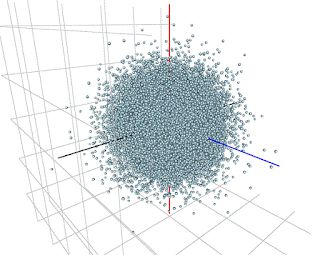
"Pickover describes a simple but quite effective technique for testing RNGs visually. The idea is to generate random numbers in groups of three, and to use each group to plot a point in spherical coordinates. If the RNG is good, the points will form a solid sphere. If not, patterns will appear. 

When it is used with good RNGs, the results of the Pickover Test are rather boring: it just draws spheres. The test is much more effective when it is used with a bad RNG, because it produces pretty pictures." 

Peter provides some nice examples of such pretty pictures!

I thought that it would be interesting to apply the Pickover Test to random numbers produced by the (default) RNG's for various distributions in R.

Before looking at the results, note that is the support of the distribution in question is finite (e.g., the Beta distribution), then the "solid sphere" that is referred to in the Pickover Test will become a "solid box". Similarly, if the support of the distribution is the real half-line (e.g., the Chi-Square distribution), the "solid sphere" will become a "solid quarter-sphere".

You can find the R code that I used on the code page that goes with this blog. Specifically, I used the "rgl" package for the 3-D plots.

Here are some of my results, in each based on a sequence of 33,000 "triplets" of random numbers:

(i) Standard Normal (using "rnorm")

(ii) Uniform on [0 , 1] (using "runif")

(iii) Binomial [n = 100, p = 0.5] (using "rbinom")

(iv) Poisson [mean = 10] (using "rpois")

(v) Standard Logistic (using "rlogis")

(vi) Beta [1 , 2] (using "rbeta")

(vii) Chi-Square [df = 5] (using "rchisq")

(vii) Student-t [df = 3] (using "rt")

(viii) Student-t [df = 7] (using "rt")

(Note that if you run my R code you can rotate the resulting 3-D plots to change the viewing aspect by holding the left mouse key and moving the mouse. You can zoom in and out by "scrolling".)

On the whole, the results look pretty encouraging, as you'd hope! One possible exception is the case of the Student-t distribution with relatively small degrees of freedom.

Of course, the Pickover "Test" is nothing more than a quick visual aid that can alert you to possible problems with your RNG. It's not intended to be a substitute for more formal, and more specific, hypothesis tests for the distribution membership, independence, etc., of your random numbers..

References

Adler, D., D. Murdoch, et al., 2017' 'rgl' package, version 0-98.1.

Pickover, C., 1995. Keys to Infinity. Wiley, New York.


© 2017, David E. Giles

Monte Carlo Simulations & the "SimDesign" Package in R

Past posts on this blog have included several relating to Monte Carlo simulation - e.g., see here, here, and here.

Recently I came across a great article by Matthew Sigal and Philip Chalmers in the Journal of Statistics Education. It's titled, "Play it Again: Teaching Statistics With Monte Carlo Simulation", and the full reference appears below.

The authors provide a really nice introduction to basic Monte Carlo simulation, using R. In particular, they contrast using a "for loop" approach, with using the "SimDesign" R package (Chalmers, 2017). 

Here's the abstract of their paper:

"Monte Carlo simulations (MCSs) provide important information about statistical phenomena that would be impossible to assess otherwise. This article introduces MCS methods and their applications to research and statistical pedagogy using a novel software package for the R Project for Statistical Computing constructed to lessen the often steep learning curve when organizing simulation code. A primary goal of this article is to demonstrate how well-suited MCS designs are to classroom demonstrations, and how they provide a hands-on method for students to become acquainted with complex statistical concepts. In this article, essential programming aspects for writing MCS code in R are overviewed, multiple applied examples with relevant code are provided, and the benefits of using a generate–analyze–summarize coding structure over the typical “for-loop” strategy are discussed."

The SimDesign package provides an efficient, and safe template for setting pretty much any Monte Carlo experiment that you're likely to want to conduct. It's really impressive, and I'm looking forward to experimenting with it.

The Sigal-Chalmers paper includes helpful examples, with the associated R code and output. It would be superfluous for me to add that here.

Needless to say, the SimDesign package is just as useful for simulations in econometrics as it is for those dealing with straight statistics problems. Try it out for yourself!

References

Chalmers, R. P., 2017. SimDesign: Structure for Organizing Monte Carlo Simulation Designs, R package version 1.7.

M. J. Sigal and R. P. Chalmers, 2016. Play it again: Teaching statistics with Monte Carlo simulation. Journal of Statistics Education, 24, 136-156.

© 2017, David E. Giles

Jan Kiviet's Book on Monte Carlo Simulation

Monte Carlo simulation is an essential tool that econometricians use a great deal. For an introduction to some aspects of Monte Carlo simulation, see my earlier posts here, here, and here. There are some follow-up posts on this coming up soon.

In the meantime, I was delighted to learn recently about an outstanding book on this topic by Jan Kiviet. The book is titled, Monte Carlo Simulation for Econometricians, and I strongly recommend it.

Of course, Jan's work will be familiar to many readers of this blog, and this book more than lives up to our expectations, given the author's excellent reputation.

Jan uses EViews to illustrate the various issues that are discussed in his book, making the material very accessible to students and researchers alike. 

This is a really nice contribution!

© 2017, David E. Giles

Monte Carlo Simulation Basics, III: Regression Model Estimators

This post is the third in a series of posts that I'm writing about Monte Carlo (MC) simulation, especially as it applies to econometrics. If you've already seen the first two posts in the series (here and here) then you'll know that my intention is to provide a very elementary introduction to this topic. There are lots of details that I've been avoiding, deliberately.

In this post we're going to pick up from where the previous post about estimator properties based on the sampling distribution left off. Specifically, I'll be applying the ideas that were introduced in that post in the context of regression analysis. We'll take a look at the properties of the Least Squares estimator in three different situations. In doing so, I'll be able to illustrate, through simulation, some "text book" results that you'll know about already.

If you haven't read the immediately preceding post in this series already, I urge you to do so before continuing. The material and terminology that follow will assume that you have.

Monte Carlo Simulation Basics, II: Estimator Properties

In the early part of my recent post on this series of posts about Monte Carlo (MC) simulation, I made the following comments regarding its postential usefulness in econometrics:

".....we usually avoid using estimators that are are "inconsistent". This implies that our estimators are (among other things) asymptotically unbiased. ......however, this is no guarantee that they are unbiased, or even have acceptably small bias, if we're working with a relatively small sample of data. If we want to determine the bias (or variance) of an estimator for a particular finite sample size (n), then once again we need to know about the estimator's sampling distribution. Specifically, we need to determine the mean and the variance of that sampling distribution. 

If we can't figure the details of the sampling distribution for an estimator or a test statistic by analytical means - and sometimes that can be very, very, difficult - then one way to go forward is to conduct some sort of MC simulation experiment."

Before proceeding further, let's recall just what we mean by a "sampling distribution". It's a very specific concept, and not all statisticians agree that it's even an interesting one.

Monte Carlo Simulation Basics, I: Historical Notes

Monte Carlo (MC) simulation provides us with a very powerful tool for solving all sorts of problems. In classical econometrics, we can use it to explore the properties of the estimators and tests that we use. More specifically, MC methods enable us to mimic (computationally) the sampling distributions of estimators and test statistics in situations that are of interest to us. In Bayesian econometrics we use this tool to actually construct the estimators themselves. I'll put the latter to one side in what follows.

Spreadsheet Errors

Five years ago I wrote a post titled, "Beware of Econometricians Bearing Spreadsheets". 

The take-away message from that post was simple: there's considerable, well-documented, evidence that spreadsheets are very, very, dangerous when it comes to statistical calculations. That is, if you care about getting the right answers!

Read that post, and the associated references, and you'll see what I mean.

(You might also ask yourself, why would I pay big bucks for commercial software that is of questionable quality when I can use high-quality statistical software such as R, for free?)

This week, a piece in The Economist looks at the shocking record of publications in genomics that fall prey to spreadsheet errors. It's a sorry tale, to be sure. I strongly recommend that you take a look.

Yes, any software can be mis-used. Anyone can make a mistake. We all know that. However, it's not a good situation when a careful and well-informed researcher ends up making blunders just because the software they trust simply isn't up to snuff!  

© 2016, David E. Giles

Econometrics Reading List for June

Here's some suggested reading for the coming month:

• Backhouse, R. and B. Cherrier, 2016. 'It's  computerization, stupid!' The spread of computers and the changing roles of theoretical and applied economics.
• Castle, J. L., M. P. Clements, and D. F. Hendry, 2016. An overview of forecasting facing breaks. Discussion Paper No. 779, Department of Economics, University of Oxford.
• Constantini. M. and A. Sen, 2016. A simple testing procedure for unit root and model specification. Computational Statistics and Data Analysis, 102, 37-54.
• Lutkepohl, H., A. Staszewska-Bystrova, and P. Winker, 2016. Calculating joint confidence bands for impulse response functions using highest density regions. SFB 649 Discussion Paper 2016-017.
• Valadkhani, A., R. Smyth, and B. Mahoney, 2016. Asymmetric causality between Australian inbound and outbound migration tourism flows. Applied Economics, in press.
• Webel, K., 2016. A data-driven selection of an appropriate seasonal adjustment approach. Discussion Paper No. 07/2016, Deutsche Bundesbank.

© 2016, David E. Giles

Econometric Computing in the Good Ol' Days

I received an email from Michael Belongia, who said:

"I wrote earlier in response to your post about Almon lags but forgot to include an anecdote that may be of interest to your follow-up.

In the late 1960s, the "St. Louis Equation"  became a standard framework for evaluating the relative effects of monetary and fiscal policy. The equation was estimated by the use of Almon lags (see, e.g., footnotes 12 and 18 in the article).  To estimate the equation, however, the St. Louis Fed had to use the computing power of nearby McDonnell-Douglas!!!  As Keith Carlson, who was in the Bank's Research Dept at the time, confirmed for me:   

'We did send our stuff out to McDonnell-Douglas.  Gave the instructions to the page who took it to the Cotton Belt building at 4th and Pine and the output would be picked up a couple days later. We did this until about 67 or 68 when we shifted to in-house.  In fact we hired the programmer from M-D.'

Difficulties like this certainly made economists of the era think more carefully about their models before taking them to the data."

I concur wholeheartedly with Michael's last comment. My own computing experience began in the late 1960's - I've posted about this in the past in The Monkey Run.

And I haven't forgotten the follow-up post on Almon distributed lag models that I promised!

© 2016, David E. Giles

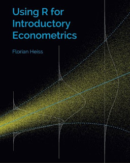
"Using R for Introductory Econometrics"

Recently, I received an email from Florian Heiss, Professor and Chair of Statistics and Econometrics at the Henrich Heine University of Dusseldorf.

He wrote:

"I'd like to introduce you to a new book I just published that might be of interest to you: Using R for Introductory Econometrics.

The goal: An introduction to R that makes it as easy as possible for undergrad students to link theory to practice without any hurdles regarding material, notation, or terminology. The approach: Take a popular econometrics textbook (Jeff Wooldridge's Introductory Econometrics) and make the whole thing as consistent as possible.

I introduce R and show how to implement all methods Wooldridge mentions mostly using his examples. I also add some Monte Carlo simulation and present tools like R Markdown.

The book is self-published, so I can offer the whole text for free online reading and a hard copy is really cheap as well."

The link for the online version of Florian's book is http://www.urfie.net/.

What you`ll find there are two versions of his 365-page book (Flash and HTML5) that you can read online; and all of the related R files for easy download.

Florian has used the CreateSpace publishing platform to produce an extremely professional product.

Using R for Introductory Econometrics is a fabulous modern resource. I know I'm going to be using it with my students, and I recommend it to anyone who wants to learn about econometrics and R at the same time.

If you're after a hard copy of the book you can purchase it for the bargain price of US$26.90 directly from CreateSpace, or from Amazon.

© 2016, David E. Giles

Gretl Update

The Gretl econometrics package is a great resource that I've blogged about from time to time. It's free to all users, but of a very high quality. 

Recently, I heard from Riccardo (Jack) Lucchetti - one of the principals of Gretl. He wrote:

"In the past, you had some nice words on Gretl, and we are grateful for that.

Your recent post on HEGY made me realise that you may not be totally aware of the recent developments in the gretl ecosystem: we now have a reasonably rich and growing array of "addons". Of course, being a much smaller project than, say, R, you shouldn't expect anything as rich and diverse as CRAN, but we, the core team, are quite pleased of the way things have been shaping up."

The HEGY post that Jack is referring to is here, and he's quite right - I haven't been keeping up sufficiently with some of the developments at the Gretl project. 

There are now around 100 published Gretl "addons", of "function packages". You can find a list of those currently supported here. By way of example, these packages include ones as diverse as Heteroskedastic I.V. Probit; VECM for I(2) Analysis; and the Moving Blocks Bootstrap for Linear Panels.

If you go to this link you'll be able to download the Gretl Function Package Guide. This will tell you everything you want to know about using function packages in Gretl, and it also provides the information that you need if you're thinking of writing and contributing a package yourself.

Congratulations to Jack and to Allin Cottrell for their continuing excellent work in making Grelt available to all of us!

© 2015, David E. Giles

Reading List for October

Some suggestions for the coming month:

• Franses, P. H., 2016. A note on the mean absolute scaled error. International Journal of Forecasting, 32, 20-22.
• Gorroochurn, P., 2015. On Galton's change from 'reversion' to 'regression'. American Statistician, in press.
• Holan, S. H., R. Lund, and G. Davis, 2010. The ARMA alphabet soup: A tour of ARMA model variants. Statistics Surveys, 4, 232-274.
• Liu, S., H. Wu, and W. Q. Meeker, 2015. Understanding and addressing the unbounded "likelihood" problem. American Statistician, 69, 191-200.
• McCracken, M. W. and S. Ng, 2015.  FRED-MD: A monthly database for macroeconomic research. Journal of Business and Economic Statistics, in press.
• Müller, U. K. and M. W. Watson, 2015. Low-frequency econometrics. NBER Working Paper No. 21564.

© 2015, David E. Giles