We all know that structural simultaneous equations models (SEM’s) played a key role in the historical development of Econometrics as a discipline. An understanding of these models and the associated estimators is an important part of our training, whether we use these models or not in our day-to-day work. The issues that they raise have helped shape much of our current econometric tool-kit.
I've posted on this topic before, but here I'm going to look at the results of applying various SEM estimators using the EViews econometrics package. In particular, I'll use a simple well-known structural model to illustrate the estimates that are obtained when different “limited information” and “full information” estimators are used.
Then, I'll take a look at using an estimated SEM for the purposes of simulating the effect of a policy shock.
The idea of constructing SEM’s for the macro. economy came from Jan Tinbergen, who estimated a 24-equation system for the Dutch economy in 1936, and others. (See Tinbergen (1959, pp.37-84) for an English translation.) When the first Nobel Prize in Economic Science was awarded in 1969, Tinbergen shared the inaugural honour with Ragnar Frisch (a Norwegian econometrician) for their pioneering work that led to the development of econometrics as a recognized sub-discipline.
Lawrence Klein was (is) also a pioneer and long-term super-star in macroeconometric modelling, for which he also won a Nobel Prize - in 1980. His work influenced econometric modelling around the world, culminating with the ambitious Project LINK.
Klein’s (1950) “Model I” for the U.S. economy was a 6-equation SEM, comprising 3 structural equations and 3 identities. The equations of Klein’s model are given below, with the endogenous variables as the dependent variables in each case:
Consumption:
Ct = α0 + α1Pt + α2Pt-1 + α3(Wpt + Wgt) + ε1t
Investment:
It = β0 + β1Pt + β2Pt-1 + β3Kt-1 + ε2t
Private Wages:
Wpt = γ0 + γ1Xt + γ2Xt-1 + γ3At + ε3t
Equilibrium Demand:
Xt ≡ Ct + Tt + Gt
Private Profits:
Pt ≡ Xt - Tt - Wpt
Capital Stock:
Kt ≡ Kt-1 + It
The predetermined variables in the model are the intercept, Gt (government non-wage spending), Tt (indirect business taxes plus net exports), Wgt (government wage bill), At (time trend, measured as years from 1931), and the lagged endogenous variables, Pt-1, Xt-1 and Kt-1. Allowing for lags, the net sample period for the estimation of the model was 1921 to 1941 inclusive.
The data for Klein's model are on the data page for this blog, and the EViews workfile that we'll be using is on the code page. Note that the variable called “K1” is just Kt-1, and “Wt” is (Wpt + Wgt).
When we estimate each of the 3 structural equations in the model by OLS, this is what we get:


Of course, given the simultaneous nature of the model, and the fact that various current-period endogenous variables appear as regressors in other equations, we know that the OLS estimator is inconsistent in this context.
So, to let's use a simple consistent estimator - Two Stage Least Squares (2SLS). This is just an instrumental variables (I.V.) estimation with all of the predetermined variables in the whole model used as the instruments. It's a "single equation" estimator, in the sense that it is applied one equation at a time.
The results that we obtain are as follows:


If you compare the OLS and 2SLS estimates of the parameters, you'll see that in some cases there are some sizeable numerical differences. Also, in almost all cases the OLS standard errors are less than their 2SLS counterparts. By using OLS, you come away with a false sense of the precision of the estimated structural coefficients.
Next, I'm going to estimate the model by Three Stage Least Squares (3SLS) – this is a “full information” or “system” estimator that has the same asymptotic efficiency as Full Information Maximum Likelihood (FIML). The advantage of this estimator over 2SLS is that not only is it consistent, but in general it will be more efficient (asymptotically) than 2SLS, as it takes into account the presence of the other equations in the model. This is done by recognizing that there will be a (contemporaneous) covariance structure between the error terms in each of the structural equations. The 2SLS estimator ignores this extra information.
We have a pretty small sample here, so let's not get too excited about results that have only asymptotic validity! Moreover, there can be a down-side to using a "system" estimator such as 3SLS. If any one of the equations in the model is mis-specified, this will render the estimates of all of the coefficients in all of the equations inconsistent. So, we should be careful in our choice of estimator.
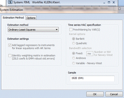
To implement 3SLS, we first need to create the system we're going to use. In the EViews workfile, we select “Object”, “New Object”, “System”. I've named the system THREESTAGE. We lay out the specification of the structural equations in the model as follows:

(To make things easy for you, if you're going to reproduce these results, the code for these equations is stored in the text-object called “Three_Stage_Spec” in the EViews workfile.)
Then we select the “Estimate” tab and choose “Three-Stage Least Squares” as the estimation method:

Pressing “OK” gives us the 3SLS estimates:

You can compare the 3SLS estimates of the parameters (and their standard errors) with their 2SLS counterparts. I'm not going to dwell on these differences here, though.
Now let’s move ahead to FIML estimation of the model. In this case the 3 identities have to be “solved out” (substituted out) from the model in order for EViews to proceed. If you don't do this, then the endogenous variables won't be distinguished properly from the predetermined variables in the likelihood function, and you'll get the wrong estimates.
With a larger SEM, this set of substitutions would be very tedious – some other econometrics packages allow you to include identities explicitly as part of the model's specification, and the substituting out of the identities is done automatically for you. It seems that this isn't the case in EViews, unfortunately.
So, in the EViews workfile, I selected “Object”, “New Object”, “System”. I named the system FIML. Then I layed out the specification of the 3 (modified) structural equations in the system as follows:

(Again, to make things easy for you if you're planning on replicating this, these equations are stored in the text-object called “FIML_Spec” in the EViews workfile.)
(Again, to make things easy for you if you're planning on replicating this, these equations are stored in the text-object called “FIML_Spec” in the EViews workfile.)
Now we select the “Estimate” tab, choose “Full Information Maximum Likelihood” as the estimation method and then select the “Options” tab. I've altered the default settings as below (including setting 1,000 as the maximum number of iterations for the maximization algorithm):


If you look at Greene (2012, p.333), or Greene (2208, p.385), you'll see a summary of the OLS, 2SLS, 3SLS and FIML results, together with some other estimates. The results there agree very closely with ours.
The estimates of the structural form parameters that we've now obtained are interesting in their own right, of course. However, we might also want to use our estimated SEM for the purposes of forecasting the endogenous variables, or for seeing how the predicted "time-path" of these variables is affected if one of the exogenous variables in the model is "shocked", to mimic a policy change of some sort.
To facilitate this, the next thing we have to do is to see how we can “solve” the estimated structural form of the SEM for the estimated restricted reduced form. In our case, the system is linear in both the endogenous variables and the parameters, so this can be achieved by straightforward matrix manipulations.
However, if the SEM were non-linear in the endogenous variables, this solution would have to be achieved iteratively as we would then have a system of non-linear equations to be solved. In that case, techniques such as the Gauss-Seidel method or Newton’s method would be used.
Note that this “solution” process has nothing to do with estimation – that's been done already. What we're now doing is converting the (estimated) structural form equations into the corresponding restricted reduced form equations so that we can either generate forecasts, or else perform policy simulations.
In EViews, there is a distinction between a "System" and a "Model". They are different types of Objects. What we've estimated is a System. We now have values (estimates) for the coefficients. There are no "unknowns". We now need to take this set of equations and store it in a form that can be manipulated. This is termed a Model.
So, first, I select “Object”, “New Object”, “Model”, and I'm going to name the new model FIML_CONTROL. There are various ways to get the estimated equations from the System into this Model. I think that the easiest way at this stage is to copy and paste our FIML System into the blank window for the FIML_CONTROL Model. We then see this:


We can then scroll through the endogenous variables to see the specifications of the other two (structural) equations in the model. (Remember that the 3 identities were substituted out of the system.)
To solve the model, we select "OK", and then click on the “Solve" tab:

Notice (top, left) that we can choose between a "Deterministic" simulation and a "Stochastic" simulation. The first of these involves just solving out for the restricted reduced from equations, and setting the error terms to zero (their mean value). This will generate a single predicted time-path for each endogenous variable.
A "Stochastic" simulation, on the other hand, recognizes the presence of the error terms. Random drawings are made for the values of the error term (you can choose how many), and then many time- paths are predicted for each endogenous variable. The mean and standard deviation of these paths is computed for every endogenous variable. What you then see is the mean path and a confidence band.
I'm just going to stick with a deterministic simulation here.
You'll also see (middle, left) that we can choose between a "Dynamic Solution" of the model, and a "Static Solution". These correspond to the dynamic and static forecasts that you can generate from an OLS regression if one or more lagged values of the dependent variable appear among the regressors.
In other words, a static solution always uses the actual values of lagged endogenous variables when generating the simulation time-paths. A dynamic solution uses the predicted (simulated) values of these variables. In practice, if we were predicting beyond the end of the sample, we'd have to use a dynamic solution, after the first prediction period. A dynamic solution is more "realistic".
For the record, the "Fit" option just reproduces the within-sample predictions, equation-by-equation, ignoring the fact that the equation is actually part of a system.
When we select “OK”, we see:

If you look at the main EViews workspace, you'll see that three new variables have been created. They are CONS_0, I_0, and WP_0. These are the simulated (predicted) values of the corresponding endogenous variables.
Now I'm going to select “Proc”, “Make Graph”, and edit the window so that it looks like this:

If I select “OK”, I get a set of graphs that compares the actual series for each variable with the time-path solved out from the model:
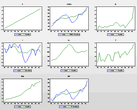
Why are there two lines on some of the graphs and only one on others? Well, in the case of variables that are exogenous there is just the (green) line for the actual data. It's only the endogenous variables that get predicted. In the latter cases there are blue lines as well, for the simulated/predicted values.
This is like looking at a plot of "Actual" and "Fitted" values for an estimated single equation regression. However, in our case, the "fitted" values take full account of the simultaneity of the system. The (within-sample) predicted values in the graphs above are produced by the restricted reduced form of the model.
What does the word “Baseline” refer to in the legends? It reflects that the simulated time-paths from the model are based on the same data that were used to estimate the system. Nothing has been tinkered with, in contrast to what we're about to see next.
Finally, let’s simulate the effect of a simple policy change. Specifically, we're going to see what the model predicts would have happened if Government Non-Wage Spending (G) had been 5 units larger (than it actually was) in each of the years 1937 to 1941 inclusive.
What follows shows how to conduct a dynamic/deterministic simulation and compare the “policy-on” (new "scenario") results with both the “policy off” “(control”, or “baseline”) results and the actual data. You can experiment with other types of simulations.
In the Model window, when we select the “Scenarios” tab, we see:

What we need to do now is to create a second version of the variable G - one that incorporates the policy change. This will provide the information needed to simulate the model under a scenario different from the "baseline" case - called "Scenario 1", here.
To do this, we first create and highlight Scenario 1, as shown above, and press “OK”. Then, in the Model window, we select the “Variables” tab, and we see:
To do this, we first create and highlight Scenario 1, as shown above, and press “OK”. Then, in the Model window, we select the “Variables” tab, and we see:

Next, we need to right-mouse-click on the variable “g”, and select “Properties”. We check the “override” box as shown below, and press the “Select Override = Actual” button:

A new variable, "G_1", has now been created in the Workfile. Right now, its identical to the original "G" variable, but we're about to change that.
We edit the series “G_1”by increasing each of the last five values by 5 units. (e.g., the 1941 value will now be 18.8.):

If we now solve the model, using "G_1" instead of "G", we'll be simulating a "policy-on" scenario. To do this, we select the “Solve” tab in the Model window and we see:

We edit the series “G_1”by increasing each of the last five values by 5 units. (e.g., the 1941 value will now be 18.8.):
If we now solve the model, using "G_1" instead of "G", we'll be simulating a "policy-on" scenario. To do this, we select the “Solve” tab in the Model window and we see:
Selecting “OK”, gives us:

The simulation has been completed, and now we want to see the results. So, we select “Proc”, “Make Graph” and edit the window as follows:

Finally, we select “OK”, and we have the graphs:

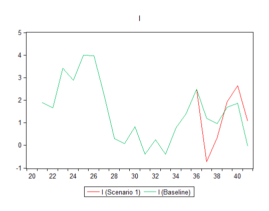
In these graphs we're able to compare the "Baseline" simulation on the model with the "Scenario 1" solution. For each of the three endogenous variables we see that when the exogenous variable, "G", is increased for the period 1937 to 1941, the predicted time-path changes. The Baseline simulation paths are in green and the "Policy-on" (Scenario 1) are in blue.
We see that an increase in Government expenditure leads to an increase in private consumption expenditure and private wages (in the top and bottom graphs) respectively. The impact on private fixed investment is more complicated (in the middle graph).
Let's look at a "blow up" of that chart, with a colour change to make things more visible:
We can go back to the System I previously called FIML. I'm going to pull up that system again, but this time I'm going to us OLS estimation:
Have fun!
References:
Greene, W. H., 2008. Econometric Analysis, 6th ed. Pearson Prentice Hall, Upper Saddle River, NJ.
Greene, W. H., 2012. Econometric Analysis, 7th ed. Pearson Prentice Hall, Upper Saddle River, NJ.
Klein, L. R., 1950. Economic Fluctuations in the United States. 1921-1941. Wiley, New York.
Tingbergen, J., 1959. Selected Papers. L. H. Klaassen, L. M. Koyck and J. H. Witteveen (eds.). North-Holland, Amsterdam.
© 2012, David E. Giles
Very helpful post Dr. Giles! However, I cannot find the attached EViews workfile in the Code Page?
ReplyDeleteSorry! It's there now.
DeleteExcellent post! I wonder if you might help me where I got stuck. In my own dataset, I have three equations and one identity (which as you said I can't explicitly include). What I did was just left the identity out, and just as you promised, when I get to the step of "converting" the system to a model, eViews seems to think there are only 3 endogenous variables where there should be 4.
ReplyDeleteMy question is that oddly, the coefficient estimates are identical to those from gretl, where I can specify the endogenous variables in a system. So even though eViews thought my price variable was exogenous, it still estimated everything fine--any idea what's going on here?
Trevor - thanks for the comment. Not sure what to suggest about this - it seems very odd. You'll see in my application I didn't just drop the identity, I substituted it into the model, thereby eliminating a variable. So the identity is actuallly fully taken into account. Not sure if this helps.
DeleteYes, I'm not sure what's going on either. I should mention this was for the TSLS estimation, not the FIML. Maybe it's not necessary to substitute in the identity for TSLS? But if that's the case, how do I force eViews to treat my 4th variable as endogenous?
DeleteTrevor - OK. if it's 2SLS, then the identity is irrelevant for ESTIMATION purposes, simply because the sample data already satisfy the identity for each observation.
DeleteYou second point - I'll have to look at that - it has to be possible as it's an obvious thing to want to do for simulation purposes.
Thanks, Dave. If you come across a way to mark a variable as endogenous I'd appreciate it--you're right, it is the obvious thing to do for forecasting/simulation.
DeleteIn case anyone stumbles across this discussion, I've learned how to 'trick' EViews into making a variable endogenous. The key is to list it first in an equation, even if it doesn't belong first in that equation. For instance, to specify that price is endogenous in a standard supply/demand system, you could write:
ReplyDeleteprice*0 + demand = f*(price + x)
See the discussion here: http://forums.eviews.com/viewtopic.php?f=10&t=6986#p24759
Trevor - thanks VERY MUCH for that!!
DeleteDG
Prof. Giles,
ReplyDeleteWhen I estimate a SEM by 2SLS, IV, or GMM do I need
to have a high r-squared and check for multicollinearity
to judge that the model is any good?
Thanks.
Multicollinearity is a data issue (a shortage of relevant information), so it is relevant regardless of the estimator you are using. R-squared are still interesting when you're using estimators other than OLS, but keep in mind that this statistic has limited appeal in any case. You shouldn't compare R-squared values across different estimators.
DeleteProf. Giles,
DeleteThank you for the clarification. I asked you the question because Gujarati's book (2012) is not very clear to me when he said that R-squared does not have the same interpretation in IV regression and could even be negative.
That's correct. The usual additive partitioning of the total sum of squares into the explained sum of squares and residual sum of squares doesn't hold once we move away from OLS (with an intercept included). With IV, etc, you get differnt R2 values if you define it as the ratio of explained SS to total SS; as opposed to defining it as 1 - (residual SS / total SS).
DeleteALways keep in mind that if you are using time series data, it is very easy to get a "high" R2 value, just because of the trends in the data. I usually don;t pay a great deal of attention to the R2 value - I'm more interested in the significance of the regression coefficients, for example.
Prof. Giles,
DeleteGreat explanation as always! Thanks!
Prof Dave
DeleteDoes Eviews software has built in function to estimate sample selection model in Full Information Maximum Likelihood method as demonstrated for the time series data here.
Advance thanks for your valuable information?
No, not for FIML estimation of a SYSTEM of equations. However, EViews 8 does have a built-in function for ML estimation of a single equation with sample selection.
Deleteprof Giles,
ReplyDeletei am running a 3sls system:
cgt= c(1)+ c(2)*nb+ c(3)*sh+ c(4)*tc+ c(5)*oil+ c(6)*o_f
nb= c(7)+ c(8)*sh+ c(9)*tc+ c(10)*o_f+ c(11)*fx
sh= c(12)+ c(13)*nb+ c(14)*tc+ c(15)*lib+ c(16)*o_f
inst tc oil o_f lib fx
how do i know which intruments to use, because my resuls are not at all what i expected.
You are using the correct instruments already if you are using either 2SLS or 3SLS. Perhpas you model is mis-specified? If you are using time-series data, perhaps some series are non-stationary?
DeleteDear prof Giles,
ReplyDeletethank you very much for your great insights. I have a question about the consmuption time series you used in this example. I ran a unit-root test and consumption definitively has a unit-root; however, you do not use first differences to make it stationary. Doesn't this affect the validity of the results? Thanks in advance!
Daniele - thanks for the comment. This is Klein's model and data from 1950, not mine. They didn't know about testing for unit roots back then!! Having said that, you could test the other variables for unit roots, AND FOR COINTEGRATION. If the data are cointegrated then, of course, we can still work with the levels, Indeed, we shouldn't difference the data unless we're going to estimate an ECM. If just some of the variables are I(1), and there is no cointegration, then the variables should be differenced to make sure that we have a "balanced" regression. You could also difference the stationary variables in this case, if this makes sense economically - differencing an I(0) variable does not leave it I(0), but it IS still stationary.
DeleteDear Dr. Giles,
ReplyDeleteThank you for this insightful post. I was hoping you could help me with a SEM model I am trying to use for simulation the fiscal/labor impact of a labor demand shock to a county in Texas.
I am trying to run a 3sls estimation in STATA for the following 14 linear equation SEM model (it is a labor/fiscal impact model known as SAFESIM) for cross-sectional labor/fiscal data for all counties in Texas. Can I put all 14 equations in to one SEM model, assuming STATA says the equations are identified and meet order conditions? I am confused as based on what I have read this model contains equations that are not autonomous (i.e. for equation 2 it makes no sense to estimate the impact of place of work employment on population, holding net-commuting fixed, as the two variables should both change in response to the labor demand shock ). Another example is equation 14, where I cannot hold fixed the property tax base per student, while estimating the impact of a change in students on state funding to school districts (because the former explanatory variable is an accounting function of the latter explanatory variable).
Additionally, I am having trouble interpreting the results if I simulate an exogenous shock of 50 new workers to the actual place of work employment. Given that these are simultaneous equations for cross-sectional data where place-of-work employment and net-commuting should change in response to the shock, I am confused what to plug in to equation 2. Would I plug in to eq. 2 for place of work employment its initial value + 50 new workers, and net-commuting would be the actual net-commuting, prior to the shock? Or would I plug in to eq. 2 for net commuting the sum of actual net commuting + the predicted change to net commuting in eq 1 resulting from the 50-unit shock to place of work employment?
1. net-commuting = f (place-of-work county employment level, county unemployment level, rural dummy)
2. population = f (place-of-work county employment, net-commuting, rural dummy)
3. civilian labor force = f (population, unemployment level, rural dummy)
4. total school-age children in county = f (population, unemployment level, hispanic population level, rural dummy)
5. total county income= f (population, county earnings, net-commuting, rural dummy)
6. retail sales & service receipts = f (total income, net-commuting, rural dummy)
7. hotel receipts == f ( total income, rural dummy)
8. mixed beverage receipts = f (total income, rural dummy)
9. total residential property value = f (total income, rural dummy
10. total commercial property value = f (total income, rural dummy)
11. intergovernmental revenue = f (population, poverty rate, rural dummy)
12. county revenue = f (property value residential, prop. val. commercial, hotel + beverage receipts, rural dummy)
13. total county expenditures = (population, total income, rural dummy)
14. total state funding to county school districts = f (total students, property tax base per student)
Thank you very much for your time.
Best,
Nabil
Respected Dave
ReplyDeleteyour post is too informative. i need a clarification. if data have mix i.e I(0) and I(1) in this case can we apply 3sls on data?
No - your data all need to be stationary; or else they all need to be I(1) and cointegrated.
DeleteRespected Dave Once again thanks for answering.If data is mix stationary i.e. I(0) and I(1) and system is simultaneous with error terms are correlated than what i can do?which estimator is proper? or how can i transform my data into the form which is suitable for 3sls?
ReplyDeleteGul - You'll have to first-difference the I(1) series.
DeleteRspected Dave
ReplyDeletewhen i try to estimate 3sls the e-view8 give error message "Near Singular Matrix".
my system of equation are as:-
SE=-c(5)*CEt+c(4)*SEt+(1-c(4))*(c(1)*TR+c(2)*A1+c(3)*A2)
CE=c(4)*c(1)*TR+c(4)*c(2)*A1+c(4)*c(3)*A2-c(4)*SEt+c(5)*CEt
DE=(1-c(9))*((1-c(1))*TR+(1-c(2))*A1+(1-c(3))*A2)+c(9)*DEt
TR=(1-c(1))*c(7)*(DE-(1-c(2))*A1-(1-c(3))*A2)-c(1)*c(8)*(SE-SEt)+c(6)*TRt
inst c a1 a2 set(-1) cet(-1) trt(-1) det(-1)
what are the reasons why this error appear and whats its mean. And finally how i resolve this issue.
You can't have the same variable on both the left side and right side of an equation, no matter what estimator you use. If it's a system estimator, the covariance matrix of the errors will be singular. It makes no logical sense to do this at any time.
DeleteGood day Professor Giles,
ReplyDeleteI noticed that you didn't run any diagnostic tests for your estimations. In particular, I'm interested in the diagnostic tests for 3sls. How do you know that your model is stable, free from heterskedasticity or free from autocorrelation? I can't seem to find any option in eviews to check for these things.
Thanks in advance for your advice.
Sakura: for 3SLS or FIML, you can VIEW the residual diagnostics and this will give you a portmanteau test for serial independence. You can save the residuals of each equation The regress a residuals series against just an intercept. The residua;ls from this artificial regression will be the same as the dependent variable but you can then VIEW the stability tests. The homoskedasticity tests are a bit more difficult - you will have to construct them manually using the 3SLS or FIML residuals for each equation.
DeleteThanks a lot Professor Giles. I'll put your advice to good use.
ReplyDeleteHi Professor Giles,
ReplyDeleteThanks for such a great topic and sharing your expertise in econometrics among other subjects. Multiple topics have been of great assistance to me during the empirical analysis of my dissertation. I work from off campus. Thanks again for your hard work. Sean Byrne
Sean - you're welcome. I've "met" a lot of great people since starting the blog.
DeleteProfessor Giles,
ReplyDeleteLet's say I have a system of equations with no contemporaneous endogenous variable (I only have exogenous variables and lagged endogenous variables as regressors). In that case, do I have to run the methods you dwell on (2SLS/3SLS...)?
Thanks
Romain
Romian - you can just estimate each equation by OLS. You can improve the estimator efficiency by using the Seemingly Unrelated Regression estimator.
DeleteProfessor Giles I stumbled on this website and I find your articles interesting. I am replicating Berndt and Wood (1975) for 1947-1971.
ReplyDeleteI prepared the following system Go_1=C(1)+c(2)* pk1 + c(3) * pl1 + c(4)* PE1+ c(5) *Pm1+.5*c(6)*(pk1*pk1)+c(7)*(pk1*pl1)+c(8)*(pk1+pe1)+c(9)*(pk1*pm1)+.5*c(10)*(pl1*pl1)+c(11)*(pl1*pe1)+c(12)*(pl1*pm1)+.5*c(13)*(pe1*pe1)+c(14)*(pe1*pm1)+.5*c(15)*(pm1*pm1)
@inst Pop work Excise prop gdur gndur Glabor realdu realndur cap (instruments)
K= c(16)+c(17)*pk1+c(18)*pl1+c(19)+pe1+c(20)*pm1
L= c(21)+c(22)*pk1+c(23)*pl1+c(24)+pe1+c(25)*pm1
E= c(26)+c(27)*pk1+c(28)*pl1+c(29)+pe1+c(30)*pm1
K, L, E are the market share equations. I left out the M equation. I am using 3sls and obtain a near singular matrix. I do not have same variables on both sides. I am stumped. Thanks for your inputs
Sorry, but this is not enough information for me to help you.
DeleteDG
Respected prof. Pls how do i interpret the coefficient of estimates from TSLS in Eviews output?
ReplyDeleteJust the same way that you would interpret OLS coefficient estimates. Note that the "t-statistics" should be treated as being Standard Normal (if you have a large sample size).
DeleteHello Sir,
ReplyDeleteThanks alot for writing such a useful post. Howevr, i have a question about the stationarity of the time series. I am trying to estimate an equation in which dependent variable is stationary at 2nd difference while all other variables are stationary at level or 1st difference. Will it be appropriate to use 2SLS on such data? if not, which technique should i move towards.
For 2SLS to be consistent, all of the data need to be stationary - so, you will have to transform your variables before applying 2SLS.
DeleteThanks for your prompt reply. After transformation, all of my variables are stationary at first difference with constant. is 2SLS correct to use now?
DeleteIf all of your series have been transformed appropriately to make them stationary, then the 2SLS estimator will be consistent.
Delete