This post comes at the request of Francesca, in a comment on an earlier post on Monte Carlo simulation.
The request was for some examples of how we can compute finite-sample critical values for different test statistics. What this really means is that we want to simulate particular "quantiles" (points on the X-axis) for the distribution of the statistic.
Let's see what we can do about this. First, some background information.
It's often the case that we know the form of the sampling distribution of our test statistic if the sample size is very large. That is, we know the asymptotic sampling distribution. However, if we're applying the test with a sample that's relatively small, we have to be careful because the actual sampling distribution of our statistic can be very different from its asymptotic distribution.
If that's the case, then the correct critical values can be quite different from the ones that we'd get if we chose them on the assumption that the asymptotic distribution is appropriate. This, in turn, will imply that we'll be using a significance level that's different from what we want!
To make matters worse, there's no simple answer to the question: "How big does the sample size have to be before we can rely on the use of the asymptotic distribution of our test statistic?" It depends on the context of the testing problem, and usually it also depends on the (unknown) values of the parameters in the problem, and on the nature of the data we're using.
So, we may not even know that we're in trouble when we rely on asymptotic results. However, we can usually simulate the situation at hand, and find out!
Perhaps a picture will help.
If we assumed that the sampling distribution for our test statistic is standard normal, and we had in mind a 5% significance level, we'd reject the null hypothesis, in favour of a positive one-sided alternative hypothesis, if our test statistic exceeded 1.645. However, if the sampling distribution is actually Student's-t, with v = 3 degrees of freedom, by using a critical value of 1.645 we would actually be using a significance level greater than the desired 5%. The tail area under the blue density exceeds that under the red density. That's the size distortion.
Now let's consider some examples that will illustrate all of this for some common tests in econometrics.
Example 1
This example involves simulating the critical values for a t-test in a regression model when the errors are far from being normally distributed. Contrary to what a lot of students get taught, normal errors are only a sufficient (but not necessary) condition for the t-statistic to be Student's-t distributed in finite samples. I discussed this point in some detail in an earlier post.
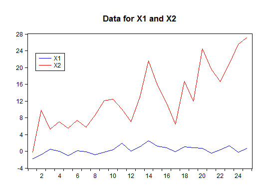
Here, I'm going to simulate the effect of the error being uniformly distributed. The simulation will involve a simple regression model, with an intercept and one other regressor. However, we'll consider two forms for this regressor: X1 will be standard normally distributed; and X2 will be a linear trend with a normal "noise" component super-imposed on it. These two series are shown below, and we'll be interested in whether or not our results are sensitive to the form of these data.
The basic version of the EViews program that I've written appears below. You'll see that there are actually only 5 lines of code for the Monte Carlo loop. In this example, I'm using the X1 regressor, a sample size of n = 500, and 10,000 Monte Carlo replications. The value of the coefficient of X1 (called "b1" in the code) is set to zero for the purposes of generating the random "y" data. So, when it comes to the t-test of H0: β1 = 0 vs. H1: β1 > 0, we're dealing with the situation where the null hypothesis is actually true. This is what we want when simulating critical values. These values are quantiles of the distribution of the test statistic, conditional on H0 being true.
The code is in three blocks: the first block just initializes some quantities we're going to use; the second block is the MC loop; and the third block sorts the 10,000 simulated t-statistics so we can find the desired right-tail quantiles (90%, 95%, and 99%).
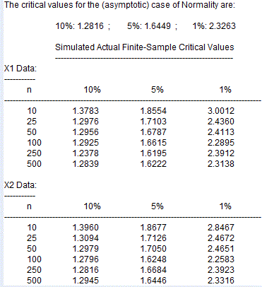
As you can see, the results depend to some degree on the form of the X data. This is a pretty standard result in experiments of this type - e.g., see King and Giles (1984). In small samples, if we were to use the asymptotic critical values as an approximation, we'd be using critical values that are "too small".
[As an exercise, you can also compare these simulated critical values with the critical values that you'd use if you treated the t-statistic as being Student's-t distributed, even though it doesn't quite follow that distribution in small samples here. For instance, when n = 10, we have 8 degrees of freedom, and in that case the 10%, 5%, and 1% critical values are 1.3968, 1.8595, and 2.8965 respectively.]
Because the asymptotic critical values are "too small", it follows that if we were to use them, the significance levels that they would imply would be larger than what we thought we were using. We usually call the intended significance level the "nominal significance level" or "nominal size" of the test. This stands in contrast to actual significance level (rejection rate) associated with using the "wrong" critical value. The difference between these two quantities is the degree of "size distortion" that we incur by wrongly using the asymptotic critical values.
I've extended the program to simulate these actual significance levels. This program, and the associated EViews workfile, are on the code page for this blog. As expected, when n is small, the actual sizes of the test exceed the nominal sizes. We can see this in the following table.
Just for interest, here's the simulated sampling distribution for on of the cases considered. It's clear from the Jarque-Bera test that the distribution is non-normal. If it were Student's-t distributed with 8 degrees of freedom, the standard deviation would be 1.155 and the kurtosis would be 4.5.
Example 2
This example involves a slightly more complex situation, but the methodology I've adopted is the same as for the first example. Once again, the EViews program and workfile are on the code page for this blog.
In this example, we're estimating a model that's non-linear in the parameters:
yi = β1 + (β2 x3i) β1 + εi ; i = 1, 2, ...., n .
The error term is normally distributed, with a zero mean. However, the usual t-test statistics won't be Student's-t distributed in finite sample. Asymptotically, these statisitcs will follow a standard normal distribution.
To complicate things further, let's consider two cases - (i) Homoskedastic errors, with var.(εi) = 1; and (ii) Heteroskedastic errors, with var.(εi) = exp(zi), where zi ~ N[0 , 1]. In the heteroskedastic case, in particular, the t-statistics will have sampling distributions that are rather messy.
In the program (which you can open using any text editor), you'll see that the true value of β2 is five, and the null hypothesis is H0: β2 = 5. Again, I've considered a positive one-sided alternative hypothesis. Here's a small selection of results for the critical values needed to ensure 10%, 5%, and 1% significance levels, for various sample sizes:
It's pretty clear that using the asymptotic (standard normal) critical values would lead to very misleading results. Just how misleading those results would be, in terms of size distortion, can be seen in the next table:
When the errors are heteroskedastic, quite a large sample is need before we can assume that the asymptotics have "kicked in". Finally, the following illustrative sampling distribution reveals the nature of the non-normality when n = 50:
Now, it's very important to note that these results are specific to the choices that I've made with respect to parameter values, data, and sample sizes. However, I think they answer Francesca's request.
What can we do in practice to get appropriate critical values, when we don't know the true parameter values? Well, that's when we can use another simulation technique, the so-called "bootstrap" to help us. I'll prepare a separate post to deal with this in the near future.
Reference
King, M. L. and D. E. A. Giles, 1984. Autocorrelation pre-testing in the linear model: Estimation, testing and prediction. Journal of Econometrics, 25, 35-48.
© 2013, David E. Giles


Excellent page! Keep up the good work.
ReplyDelete