Osman, a reader of this blog, sent a comment in relation to my recent post on the effects of temporal aggregation on t-tests, and the like. Rather than just bury it, with a short response, in the "Comments" section of that post, I thought I'd give it proper attention here.
The comment read as follows:
"Thank you for this illustrative example. My question is not exactly related to the subject of your post. As you illustrated, the finite sample properties of tests are studied by investigating the size and power properties. You reported size distortions to assess the size properties of the test. My first question is about the level of the size distortions. How much distortions is need to conclude that a test is useless? Is there an interval that we can construct around a nominal size value to gauge the significance of distortions? Same type of questions can also be relevant for the power properties. The “size adjusted power” is simply rejection rates obtained when the DGP satisfies an alternative hypothesis. Although, the power property is used to compare alternative tests, we can still ask question regarding to the level of the power. As your power curve shows, the level of power also depends on the parameter value assumed under the alternative hypothesis. For example, when β1 = 0.8 the power is around 80% which means that the false null is rejected 80 times out of 100 times. Again, the question is that what should be the level of the power to conclude that the test has good finite sample properties?"Let's look at Osman's questions.
1. How much size distortion can we tolerate before the test is useless?
There's no simple answer to this, because the choice of the (nominal) significance level (size) of the test is totally arbitrary. It's up to you as the researcher.
On the other hand, suppose that my simulation evidence indicates that when you think you're applying the test at the 5% significance level, really the true size of the test is (say) 1%. Then, your reaction might be, "If that's the case then I'm really using a much smaller size than I can live with. That means that the probability of a Type II error is much larger than it needs to be, and so I'm actually applying the test in a way that reduces its power below what I'd like. Maybe I should use a critical value that's consistent with a (nominal) significance level of (say) 20%. Then the true size should be more like what I really want - something around 5%.
So, as I said, there's no simple answer to this question. However, knowing that there is size distortion, and in which direction, can be very helpful in terms of designing our testing strategy.
"No scientific worker has a fixed level of significance at which from year to year, and in all circumstances, he rejects hypotheses; he rather gives his mind to each particular case in the light of his evidence and his ideas. (Fisher, 1956, p. 42.)"You might decide to use 5%, 10%, 20%,....whatever. However, suppose that my simulation evidence indicates that when you think you're applying the test at the 5% significance level, really the true size of the test is (say) 20%. Then, your reaction would probably be "Yikes! I can't live with a false rejection rate of 20%! Maybe I should use a critical value that's consistent with a (nominal) significance level of (say) 1%. Then the true size should be more like what I really want - something around 5%."
On the other hand, suppose that my simulation evidence indicates that when you think you're applying the test at the 5% significance level, really the true size of the test is (say) 1%. Then, your reaction might be, "If that's the case then I'm really using a much smaller size than I can live with. That means that the probability of a Type II error is much larger than it needs to be, and so I'm actually applying the test in a way that reduces its power below what I'd like. Maybe I should use a critical value that's consistent with a (nominal) significance level of (say) 20%. Then the true size should be more like what I really want - something around 5%.
So, as I said, there's no simple answer to this question. However, knowing that there is size distortion, and in which direction, can be very helpful in terms of designing our testing strategy.
2. Is there an interval we can construct around a nominal size to gauge the significance of distortions?
3. The definition of "size-adjusted power"
Actually, the definition of size-adjusted power is not "...simply rejection rates obtained when the DGP satisfies an alternative hypothesis."
Size-adjusted power is the rate at which the null hypothesis is rejected, when it is false, and when the critical value that is used is the one that will actually ensure that there is no size distortion. That is, the critical value is altered (up or down, as needed) from that associated with the nominal significance level, to the value that ensures that the rate at which the test rejects the null hypothesis when it is true is the desired α%.
Usually, to find out what this new critical value should be requires some Monte Carlo simulation. In terms of a day-to-day application, we usually wouldn't do this. In that case, what's of interest is the "raw power" of the test - the rate at which it rejects false null hypotheses when the "wrong" critical value is used.
Size-adjusted power is of paramount importance, however, when comparing alternative tests. For a fixed sample size, we should only compare the powers of tests which have the same actual significance level. Otherwise it's an unfair comparison that favours the test with the larger significance level. If we size-adjust, we create a level playing field for the purposes of such comparisons. The only exception, really would be the following. Suppose that Test 1 has a smaller significance level than Test 2, and Test 1 has greater raw power than Test 2, for all alternative hypotheses. Then, unambiguously, Test 1 has greater power than Test 2. Thers is no need to "size-adjust" the tests to determine this.
Let's look at a simple example - one where we actually know what the small-sample distribution of the test statistic, and we also know the (large-n) asymptotic distribution. (Often, in practice, we'll know the asymptotic distribution, but not the finite-sample distribution. Then we'll apply the test as if the asymptotics hold, when really they don't, and this is where the size distortion will enter the picture.)
Specifically, consider a t-test on the mean of a Normal population. In finite samples, the test statistic follows a Student-t distribution with (n - 1) degrees of freedom, if the null hypothesis is true. (If the null hypothesis is false, then the statistic's distribution is non-central Student-t, with a "non-centrality parameter" that increases in value as the null hypothesis becomes increasingly false.) Asymptotically, the statistic's sampling distribution is Standard Normal, if the null hypothesis is true.
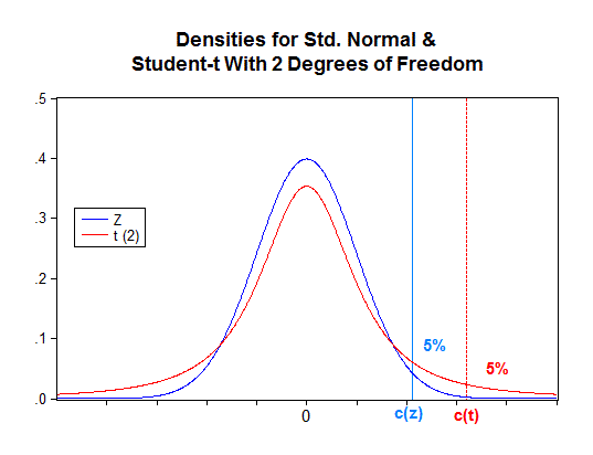
Suppose that (n - 1) = 2. Then the finite-sample and asymptotic "null distributions" for the t-statistic are as shown in the diagram above. Suppose we wanted to apply the t-test with a significance level of 5%. If we were to wrongly use the normal distribution as an "asymptotic approximation", we'd use c(z) = 1.645 as the critical value. In fact, Pr[t(2) > 1.645] = 12.09%. This is what the "actual size" of the test would be for our small sample - not the 5% we intended.
Looking at it the other way around, if we used the correct finite-sample distribution, the 5% critical value for the t-test is c(t) = 2.92. That is Pr[t(2) > 2.92] = 5%. To achieve this result if we were using our z-approximation, we'd actually have to use a "nominal" significance level of 0.18%, (not 5%) because Pr[z > 2.92] = 0.18%.
4. "The level of power also depends on the parameter value assumed under the alternative hypothesis"
Let's be careful here. It's not the value that's "assumed" it's the actual (but unobserved) value of that parameter. As that actual value changes, so does the power. Let's go back to t-test example above, and let's focus entirely on the finite-sample case. Forget about asymptotic approximations and the z distribution for now. When the null hypothesis is true the t-statistic has a sampling distribution that is Student-t with (n - 1) = 2 degrees of freedom. The density for that sampling distribution is shown in red in the diagram.
As I've said already, when the null hypothesis is false, and the alternative hypothesis prevails, the test statistic's sampling distribution is non-central Student-t. We're usually dealing with alternative hypotheses that are "composite" - e.g., μ > 0, or μ ≠ 0. There's an infinity of values for μ that are associated with the alternative hypothesis. The non-centrality parameter associated with the non-null distribution of the t-statistic increases monotonically with the (absolute) value of μ2. This "shifts" the red density continuously and the rejection region increases continuously in area. That is, the power of the test increases as the unknown value of μ changes.
5. "What should be the level of the power to conclude that the test has good finite sample properties?"
Again, this really isn't the right question to be asking. What we should be asking is: "How well does the power of my test compare with the powers of alternative tests, for my sample size, my chosen significance level, and for some fixed extent to which the null hypothesis is false?" If the answer to this question is that my test is more powerful, for fixed n and alpha, regardless of how false the null hypothesis is, then I'm using a test that is "Uniformly Most Powerful (UMP)".
For some testing problems, no UMP test exists. However, for many of the testing problems you'll encounter, a UMP test does exist, and this is what leads us to use certain tests that you're familiar with. For instance, the t-test is UMP when the alternative hypothesis is one-sided.
Osman - I hope that this explanation is helpful to you and other readers of this blog.
Dear Dave,
ReplyDeleteThank you for this instructive post.
Osman.
Osman - no problem. They were good questions.
Delete