Today being Mothers' Day in many parts of the world, I thought that flowers would be appropriate. Well, a price index for (Gardens, Plants, and) Flowers. Specifically, a harmonized price index for these goods for 27 European Union countries.
I retrieved the monthly data for the period January 2006 to March 2013 from Quandl.com - a really nice resource that I posted about recently. As well as downloading the data in various formats, reading the data from R, etc., you can also embed an interactive chart of the data directly into a document such as this one, and make the data visible to viewers.
I retrieved the monthly data for the period January 2006 to March 2013 from Quandl.com - a really nice resource that I posted about recently. As well as downloading the data in various formats, reading the data from R, etc., you can also embed an interactive chart of the data directly into a document such as this one, and make the data visible to viewers.
My price series is not seasonally adjusted, but it has a pronounced seasonal pattern, I thought I'd use this post to illustrate the basics of seasonal adjustment. What I'm going to do is take you through the steps associated with a bare-bones version of the ratio-to-moving-average method. This is something that I show students if I'm teaching an introductory descriptive economic statistics course.
Then, I'll show you how close the results are to the ones that you get if you seasonally adjust the data using the full-blown Census X-13 method that is employed by most statistical agencies world-wide.
Let the price index at time 't' be denoted by Pt, and let's assume that this series is made up of the product of trend (Tt), cycle (Ct), and irregular(It) components. (In fact, when I use the X13 method and allow it to decide whether the series is multiplicative or additive in its components, it selects the multiplicative model I'm using here.)
So, taking natural logarithms, we have:
ln(Pt) = ln(Tt) + ln(Ct) + ln(It) .
The rudimentary ratio-to-moving-average method involves the following steps. The column labels refer to the associated Excel workbook and csv file that are available on the data page of this blog:
- First, we take an unweighted 12-month arithmetic moving average of the ln(Pt) data. (Column D.) Averaging the data smooths the series. A 12-month average should smooth out the seasonal movements, as well as any irregular movements.
- There's a slight problem - it's to do with the "timing" of the observations in Column D. It arises because there's an even number (12) of months in a year. Conceptually, the first figures in Column D ( 4.48255) should be located half way between the June and July months if it's to be at the middle of the year. Right now, it's half a month out of alignment. This problem also arises if we're seasonally adjusting quarterly time-series data, because 4 is an even number too. (There's also an even number of weeks in a year - but I digress!)
- To re-align the data, we now take an unweighted 2-period arithmetic moving average of the numbers in Column D. The results appear in Column E. Averaging two "out-of-alignment" numbers shifts them by half a month, and bingo, they're now lined up with the appropriate dates! We call the resulting series the "Centered Moving Average".
- If we've done things properly there should be 6 values "missing" at the start of the series in Column E, and 6 missing at the end. (Two and two, if we had quarterly data.)
- What have we achieved by this? Well, the data in Column E represent what is left of the ln(Pt) series after we've smoothed away the Seasonal and Irregular components. That is, they represent the combined ln(Trend) and ln(Cycle) components.
- Next, we subtract the Centered Moving Average series (Column E) from the ln(Pt) data in Column C. This gives us (in Column F) the ln(Seasonal) and ln(Irregular) components.
- Then, we take the arithmetic mean of all of the July month values in Column F. This gives us a single, common "seasonal factor" for that month. We then do the same with all of the August month values in that column, and so on. The results appear in Column G. Notice that we're implicitly assuming that the seasonal factors are going to be stable over time.
- We're nearly there! If we add up the 12 seasonal factors they should sum to zero over the full year. Seasonality, by definition, is an intra-year phenomenon. Let's CHECK if we have this result. You can see in the workbook that they actually sum to 0.00178098. Not bad, but not good enough!
- We apportion this discrepancy across the 12 seasonal factors by subtracting (0.00178098/12) from each of the numbers in Column G. The results, which are the final seasonal factors, appear in Column H. Notice that these factors are repeated, year after year.
- We can now seasonally adjust the ln(Pt) series. We subtract these seasonal factors from the data in Column C. The results appear in Column I.
- Taking the exponential of the Column I series gives us the seasonally adjusted series for Pt itself, as in Column J. Notice that if I hadn't taken the logarithm of Pt before starting the adjustment process, I could have achieved the same results by using geometric averages in place of arithmetic averages, everywhere above; and by dividing, rather than subtracting, everywhere. In particular, at step 6 we would have isolated the "Seasonal and Irregular" components from the "Trend and Cycle" components by taking the Ratio of Pt to the centered moving average series. Hence the name of this seasonal adjustment method.
Next, I used Eviews to apply the X-13 seasonal adjustment method to Pt. Once you are viewing the series, you select "Proc", and then "Seasonal Adjustment", and go from there. Here's the original price index and its seasonally adjusted counterpart:

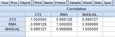
The EViews workfile that I used is on the code page for this blog. In that file there are actually three seasonally adjusted versions of the price index. The series called "X13" will be self-explanatory; the series called "Manual" was obtained using the basic steps outlined above, as shown in the Excel workbook; and the series called "RMA" was obtained using the "moving average" option under the "seasonal adjustment" procedure in EViews. The latter series should be almost identical to "Manual", and indeed it is. More on this below.
Now, how similar is my rudimentary seasonally adjusted series, "Manual", to the one obtained using X-13? Here's a scatter-plot of the two series - it's virtually a 45-degree line.

This is confirmed by the following OLS regression, and simple correlations:

You can see that there is almost a perfect correlation between my seasonally adjusted series, and both "RMA" and "X13":
The rudimentary ratio-to-moving average seasonal adjustment procedure that I went through above isn't always going to provide results that are this close to the ones that you get when you use X-13. There are several reasons for this:
- X-13 can allow for outliers in the data. Our basic method ignores this possibility.
- X-13 can allow for a seasonal pattern that "evolves" over the cycle, or over time. Our basic method assumes a stable seasonal pattern.
- X-13 can allow for the fact that different months have different numbers of "trading days", and for "holiday effects", such as the moving dates for Easter. These effects are ignored in our basic method.
- X-13 can deal with "end-point" effects that arise at the beginning and end of the sample, where values can't be computed for the centered moving averages. Our basic method doesn't take this into account.
However, in many cases, very similar seasonally adjusted series are obtained. This is very comforting for those of us who teach this material. You can take students through the rudimentary steps that I've outlined, and they can generate very convincing seasonally adjusted time-series.
Oh yes - don't forget those flowers for Mothers' Day!
Oh yes - don't forget those flowers for Mothers' Day!
© 2013, David E. Giles
Is there a reason that in column D, the 12-month MA starts in July? Isn't that a 6-month average instead?
ReplyDeleteIt's a 12-month moving average - you can verify this from the numbers. When you construct an n-period MA you "lose" observations at both the beginning and end of the series. The spreadsheet doesn't allow us to "position" a number half-way between 2 rows, which is what we'd like to do presentationally in column D. This is why a 2-period MA is then performed to "line up" the numbers with the dates for the original data. When you get to column E, you will see that there are now 6 observations missing at both the beginning and end of the series. This is correct - if you use an n-period MA, and then centre with a 2-period AM, you should have "lost" (n/2) observations at each end of the series when you are done.
DeleteDear Professor,
ReplyDeleteThank you so much for this very illustrative and pedagogical guided example (and for the excel)! Great content, still relevant nowadays.